Predicting Age in Census Data#
Introduction#
The objective of this toy project is to predict the age of an individual
with the 1994 US Census Data using multiple linear regression. We use
the Statsmodels and Patsy modules for this task with Pyhon version
>= 3.6. The dataset was sourced from the UCI Machine Learning
Repository at https://archive.ics.uci.edu/ml/datasets/adult (Lichman,
2013).
This report is organized as follows:
Overview section describes the dataset used and the features in this dataset.
Data Preparation section covers data cleaning and data preparation steps.
Data Exploration section explores dataset features and their inter-relationships.
Statistical Modeling and Performance Evaluation section first fits a full multiple linear regression model and performs diagnostic checks. Next, we perform backwards variable selection using p-values to obtain a reduced model, after which we perform another set of diagnostic checks on the reduced model.
Summary and Conclusions section provides a summary of our work and presents our findings.
Overview#
Data Source#
The UCI Machine Learning Repository provides five datasets, but only
adult.data, adult.test, and adult.names were useful in this
project. The adult.data and adult.test are the training and test
datasets respectively. The adult.names file contains the details of
the variables (a.k.a. features or attributes). The training dataset has
32,561 observations (a.k.a. instances or records) and the test dataset
has 16,281 observations. Both datasets consist of 14 descriptive (a.k.a.
independent) features and one target (a.k.a. response or dependent)
feature. In this project, we combine both training and test data into
one.
Project Objective#
Our goal is to see if we can predict an individual’s age within an acceptable margin of error using multiple linear regression primarily with just main affects.
Target Feature#
Our target feature is age, which is a continuous numerical feature.
Hence, our project is on a regression problem.
Descriptive Features#
The variable descriptions below are from the adult.names file:
workclass: Private, Self-emp-not-inc, Self-emp-inc, Federal-gov, Local-gov, State-gov, Without-pay, Never-worked.fnlwgt: continuous.education: Bachelors, Some-college, 11th, HS-grad, Prof-school, Assoc-acdm, Assoc-voc, 9th, 7th-8th, 12th, Masters, 1st-4th, 10th, Doctorate, 5th-6th, Preschool.education-num: continuous.marital-status: Married-civ-spouse, Divorced, Never-married, Separated, Widowed, Married-spouse-absent, Married-AF-spouse.occupation: Tech-support, Craft-repair, Other-service, Sales, Exec-managerial, Prof-specialty, Handlers-cleaners, Machine-op-*inspct, Adm-clerical, Farming-fishing, Transport-moving, Priv-house-serv, Protective-serv, Armed-Forces.relationship: Wife, Own-child, Husband, Not-in-family, Other-relative, Unmarried.race: White, Asian-Pac-Islander, Amer-Indian-Eskimo, Other, Black.sex: Female, Male.capital-gain: continuous.capital-loss: continuous.hours-per-week: continuous.native-country: United-States, Cambodia, England, Puerto-Rico, Canada, Germany, Outlying-US(Guam-USVI-etc), India, Japan, Greece, South, China, Cuba, Iran, Honduras, Philippines, Italy, Poland, Jamaica, Vietnam, Mexico, Portugal, Ireland, France, Dominican-Republic, Laos, Ecuador, Taiwan, Haiti, Columbia, Hungary, Guatemala, Nicaragua, Scotland, Thailand, Yugoslavia, El Salvador, Trinadad&Tobago, Peru, Hong, Holand-Netherlands.income: binary, 1: earns over \\(50k a year, 0: earns less than \\\)50k a year.
Most of the descriptive features are self-explanatory, except fnlwgt
which stands for “Final Weight” defined by the US Census. This weight is
an “estimate of the number of units in the target population that the
responding unit represents” (Lichman, 2013). This feature aims to
allocate similar weights to people with similar demographic
characteristics.
Data Preparation#
Preliminaries#
For further information on how to prepare your data for statistical modeling, please refer to this page on our website.
First, let’s import all the common modules we will be using.
# Importing modules
import numpy as np
import pandas as pd
import matplotlib.pyplot as plt
import seaborn as sns
import statsmodels.api as sm
import statsmodels.formula.api as smf
import patsy
import warnings
###
warnings.filterwarnings('ignore')
###
%matplotlib inline
%config InlineBackend.figure_format = 'retina'
plt.style.use("seaborn-v0_8")
We read the training and test datasets directly from the data URLs.
Also, since the datasets do not contain the attribute names, they are
explicitly specified during data loading process. The adultData
dataset is read first and then it is concatenated with adultTest as
just data.
# Gettting data from the web
url = (
    "http://archive.ics.uci.edu/ml/machine-learning-databases/adult/adult.data",
    "http://archive.ics.uci.edu/ml/machine-learning-databases/adult/adult.test",
)

# Specifying the attribute names
attributeNames = [
    'age',
    'workclass',
    'fnlwgt',
    'education',
    'education-num',
    'marital-status',
    'occupation',
    'relationship',
    'race',
    'sex',
    'capital-gain',
    'capital-loss',
    'hours-per-week',
    'native-country',
    'income',
]

# Read in data
adultData = pd.read_csv(url[0], sep = ',', names = attributeNames, header = None)
adultTest = pd.read_csv(url[1] , sep = ',', names = attributeNames, skiprows = 1)

# Join the two datasets together
data = pd.concat([adultData,adultTest])

# we will not need the datasets below anymore, so let's delete them to save memory
del adultData, adultTest

# Display randomly selected 10 rows
data.sample(10, random_state=999)
| age | workclass | fnlwgt | education | education-num | marital-status | occupation | relationship | race | sex | capital-gain | capital-loss | hours-per-week | native-country | income | |
|---|---|---|---|---|---|---|---|---|---|---|---|---|---|---|---|
| 77 | 67 | ? | 212759 | 10th | 6 | Married-civ-spouse | ? | Husband | White | Male | 0 | 0 | 2 | United-States | <=50K |
| 30807 | 62 | Self-emp-not-inc | 224520 | HS-grad | 9 | Married-civ-spouse | Sales | Husband | White | Male | 0 | 0 | 90 | United-States | >50K |
| 23838 | 32 | Private | 262153 | HS-grad | 9 | Divorced | Craft-repair | Unmarried | White | Male | 0 | 0 | 35 | United-States | <=50K |
| 24124 | 41 | Private | 39581 | Some-college | 10 | Divorced | Adm-clerical | Not-in-family | Black | Female | 0 | 0 | 24 | El-Salvador | <=50K |
| 22731 | 66 | ? | 186032 | Assoc-voc | 11 | Widowed | ? | Not-in-family | White | Female | 2964 | 0 | 30 | United-States | <=50K |
| 2975 | 27 | Private | 37933 | Some-college | 10 | Never-married | Adm-clerical | Unmarried | Black | Female | 0 | 0 | 40 | United-States | <=50K |
| 4457 | 31 | State-gov | 93589 | HS-grad | 9 | Divorced | Protective-serv | Own-child | Other | Male | 0 | 0 | 40 | United-States | <=50K |
| 32318 | 34 | Private | 117963 | Bachelors | 13 | Married-civ-spouse | Craft-repair | Husband | White | Male | 0 | 0 | 40 | United-States | >50K |
| 12685 | 61 | Self-emp-not-inc | 176965 | Prof-school | 15 | Married-civ-spouse | Prof-specialty | Husband | White | Male | 0 | 0 | 50 | United-States | >50K |
| 2183 | 47 | Private | 156926 | Bachelors | 13 | Married-civ-spouse | Prof-specialty | Husband | White | Male | 0 | 0 | 40 | United-States | >50K. |
Note: Alternatively, you can download the datasets from UCI
Repository as txt files to your computer and then read them in as
below.
    adultData = pd.read_csv('adult.data.txt', sep = ',', names = attributeNames, header = None)
    adultTest = pd.read_csv('adult.test.txt', sep = ',', names = attributeNames, skiprows = 1)
Data Cleaning and Transformation#
We first confirm that the feature types match the descriptions outlined in the documentation.
print(f"Shape of the dataset is {data.shape} \n")
print(f"Data types are below where 'object' indicates a string type: ")
print(data.dtypes)
Shape of the dataset is (48842, 15)

Data types are below where 'object' indicates a string type:
age                int64
workclass         object
fnlwgt             int64
education         object
education-num      int64
marital-status    object
occupation        object
relationship      object
race              object
sex               object
capital-gain       int64
capital-loss       int64
hours-per-week     int64
native-country    object
income            object
dtype: object
Checking for Missing Values¶#
print(f"\nNumber of missing values for each feature:")
print(data.isnull().sum())
Number of missing values for each feature:
age               0
workclass         0
fnlwgt            0
education         0
education-num     0
marital-status    0
occupation        0
relationship      0
race              0
sex               0
capital-gain      0
capital-loss      0
hours-per-week    0
native-country    0
income            0
dtype: int64
On surface, no attribute contains any missing values, though we shall see below that the missing values are coded with a question mark. We will address this issue later.
Summary Statistics#
from IPython.display import display, HTML
display(HTML('<b>Table 1: Summary of continuous features</b>'))
data.describe(include='int64')
| age | fnlwgt | education-num | capital-gain | capital-loss | hours-per-week | |
|---|---|---|---|---|---|---|
| count | 48842.000000 | 4.884200e+04 | 48842.000000 | 48842.000000 | 48842.000000 | 48842.000000 |
| mean | 38.643585 | 1.896641e+05 | 10.078089 | 1079.067626 | 87.502314 | 40.422382 |
| std | 13.710510 | 1.056040e+05 | 2.570973 | 7452.019058 | 403.004552 | 12.391444 |
| min | 17.000000 | 1.228500e+04 | 1.000000 | 0.000000 | 0.000000 | 1.000000 |
| 25% | 28.000000 | 1.175505e+05 | 9.000000 | 0.000000 | 0.000000 | 40.000000 |
| 50% | 37.000000 | 1.781445e+05 | 10.000000 | 0.000000 | 0.000000 | 40.000000 |
| 75% | 48.000000 | 2.376420e+05 | 12.000000 | 0.000000 | 0.000000 | 45.000000 |
| max | 90.000000 | 1.490400e+06 | 16.000000 | 99999.000000 | 4356.000000 | 99.000000 |
display(HTML('<b>Table 2: Summary of categorical features</b>'))
data.describe(include='object')
| workclass | education | marital-status | occupation | relationship | race | sex | native-country | income | |
|---|---|---|---|---|---|---|---|---|---|
| count | 48842 | 48842 | 48842 | 48842 | 48842 | 48842 | 48842 | 48842 | 48842 |
| unique | 9 | 16 | 7 | 15 | 6 | 5 | 2 | 42 | 4 |
| top | Private | HS-grad | Married-civ-spouse | Prof-specialty | Husband | White | Male | United-States | <=50K |
| freq | 33906 | 15784 | 22379 | 6172 | 19716 | 41762 | 32650 | 43832 | 24720 |
Table 2 shows the feature income has four categories (or a cardinality
of 4). It was supposed to be 2 since income must be binary. We shall
explain how to fix this cardinality issue later.
Continuous Features¶#
As discussed earlier, the fnlwgt variable has no predictive power, so
it is removed. In addition, since we have an education categorical
feature, we will go ahead and remove the education-num feature as it
relays the same information and therefore redundant.
data = data.drop(columns=['fnlwgt', 'education-num'])
data['age'].describe()
count    48842.000000
mean        38.643585
std         13.710510
min         17.000000
25%         28.000000
50%         37.000000
75%         48.000000
max         90.000000
Name: age, dtype: float64
The range of age appears reasonable as the minimum and maximum ages
are 17 and 90 respectively.
Next, we define capital = capital-gain - capital-loss and then remove
the individual gain and loss variables. The summary statistic for
capital is displayed below.
data['capital'] = data['capital-gain'] - data['capital-loss']
data = data.drop(columns=['capital-gain', 'capital-loss'])
data['capital'].describe()
count    48842.000000
mean       991.565313
std       7475.549906
min      -4356.000000
25%          0.000000
50%          0.000000
75%          0.000000
max      99999.000000
Name: capital, dtype: float64
Fixing Column Names#
Some column names contain a minus sign, which can be problematic when modeling. Basically, when we write the regression formula, a minus sign will mean “exclude this variable”, which is clearly not our intent here. For this reason, we modify the column names so that the minus signs are replaced with an underscore sign.
data.columns = [colname.replace('-', '_') for colname in list(data.columns)]
data.head()
| age | workclass | education | marital_status | occupation | relationship | race | sex | hours_per_week | native_country | income | capital | |
|---|---|---|---|---|---|---|---|---|---|---|---|---|
| 0 | 39 | State-gov | Bachelors | Never-married | Adm-clerical | Not-in-family | White | Male | 40 | United-States | <=50K | 2174 |
| 1 | 50 | Self-emp-not-inc | Bachelors | Married-civ-spouse | Exec-managerial | Husband | White | Male | 13 | United-States | <=50K | 0 |
| 2 | 38 | Private | HS-grad | Divorced | Handlers-cleaners | Not-in-family | White | Male | 40 | United-States | <=50K | 0 |
| 3 | 53 | Private | 11th | Married-civ-spouse | Handlers-cleaners | Husband | Black | Male | 40 | United-States | <=50K | 0 |
| 4 | 28 | Private | Bachelors | Married-civ-spouse | Prof-specialty | Wife | Black | Female | 40 | Cuba | <=50K | 0 |
Categorical Features#
Let’s have a look at the unique values of the categorical columns. In
Pandas, string types are of data type “object”, and usually these
would be the categorical features.
categoricalColumns = data.columns[data.dtypes==object].tolist()

for col in categoricalColumns:
    print('Unique values for ' + col)
    print(data[col].unique())
    print('')
Unique values for workclass
[' State-gov' ' Self-emp-not-inc' ' Private' ' Federal-gov' ' Local-gov'
 ' ?' ' Self-emp-inc' ' Without-pay' ' Never-worked']

Unique values for education
[' Bachelors' ' HS-grad' ' 11th' ' Masters' ' 9th' ' Some-college'
 ' Assoc-acdm' ' Assoc-voc' ' 7th-8th' ' Doctorate' ' Prof-school'
 ' 5th-6th' ' 10th' ' 1st-4th' ' Preschool' ' 12th']

Unique values for marital_status
[' Never-married' ' Married-civ-spouse' ' Divorced'
 ' Married-spouse-absent' ' Separated' ' Married-AF-spouse' ' Widowed']

Unique values for occupation
[' Adm-clerical' ' Exec-managerial' ' Handlers-cleaners' ' Prof-specialty'
 ' Other-service' ' Sales' ' Craft-repair' ' Transport-moving'
 ' Farming-fishing' ' Machine-op-inspct' ' Tech-support' ' ?'
 ' Protective-serv' ' Armed-Forces' ' Priv-house-serv']

Unique values for relationship
[' Not-in-family' ' Husband' ' Wife' ' Own-child' ' Unmarried'
 ' Other-relative']

Unique values for race
[' White' ' Black' ' Asian-Pac-Islander' ' Amer-Indian-Eskimo' ' Other']

Unique values for sex
[' Male' ' Female']

Unique values for native_country
[' United-States' ' Cuba' ' Jamaica' ' India' ' ?' ' Mexico' ' South'
 ' Puerto-Rico' ' Honduras' ' England' ' Canada' ' Germany' ' Iran'
 ' Philippines' ' Italy' ' Poland' ' Columbia' ' Cambodia' ' Thailand'
 ' Ecuador' ' Laos' ' Taiwan' ' Haiti' ' Portugal' ' Dominican-Republic'
 ' El-Salvador' ' France' ' Guatemala' ' China' ' Japan' ' Yugoslavia'
 ' Peru' ' Outlying-US(Guam-USVI-etc)' ' Scotland' ' Trinadad&Tobago'
 ' Greece' ' Nicaragua' ' Vietnam' ' Hong' ' Ireland' ' Hungary'
 ' Holand-Netherlands']

Unique values for income
[' <=50K' ' >50K' ' <=50K.' ' >50K.']
Some categorical attributes contain excessive white spaces, which makes
life hard when filtering data. We will apply the strip() function to
remove extra white spaces.
for col in categoricalColumns:
    data[col] = data[col].str.strip()
WARNING: The Statsmodels module does not play nice when you have a
minus sign in levels of categorical variables, especially when you try
to some sort of automatic variable selection. The reason is that the
minus sign has a special meaning in the underlying Patsy module: it
means remove this feature. So, we will replace all the minus signs in
categorical variable level names with an underscore sign. In addition, a
dot sign is not allowed either.
for col in categoricalColumns:
    data[col] = data[col].str.replace('-', '_')
data.head()
| age | workclass | education | marital_status | occupation | relationship | race | sex | hours_per_week | native_country | income | capital | |
|---|---|---|---|---|---|---|---|---|---|---|---|---|
| 0 | 39 | State_gov | Bachelors | Never_married | Adm_clerical | Not_in_family | White | Male | 40 | United_States | <=50K | 2174 |
| 1 | 50 | Self_emp_not_inc | Bachelors | Married_civ_spouse | Exec_managerial | Husband | White | Male | 13 | United_States | <=50K | 0 |
| 2 | 38 | Private | HS_grad | Divorced | Handlers_cleaners | Not_in_family | White | Male | 40 | United_States | <=50K | 0 |
| 3 | 53 | Private | 11th | Married_civ_spouse | Handlers_cleaners | Husband | Black | Male | 40 | United_States | <=50K | 0 |
| 4 | 28 | Private | Bachelors | Married_civ_spouse | Prof_specialty | Wife | Black | Female | 40 | Cuba | <=50K | 0 |
The workclass, occupation, and native-country features contain
some missing values encoded as “?”. These observations comprise 7.4% of
the total number of observations.
mask = (data['workclass'] == '?') | (data['occupation'] == '?') | (data['native_country'] == '?')
mask.value_counts(normalize = True)*100
False    92.588346
True      7.411654
Name: proportion, dtype: float64
We now remove the rows with missing occupation, workclass, and native-country where missing values are encoded as “?”.
data = data[data['workclass'] != "?"]
data = data[data['occupation'] != "?"]
data = data[data['native_country'] != "?"]
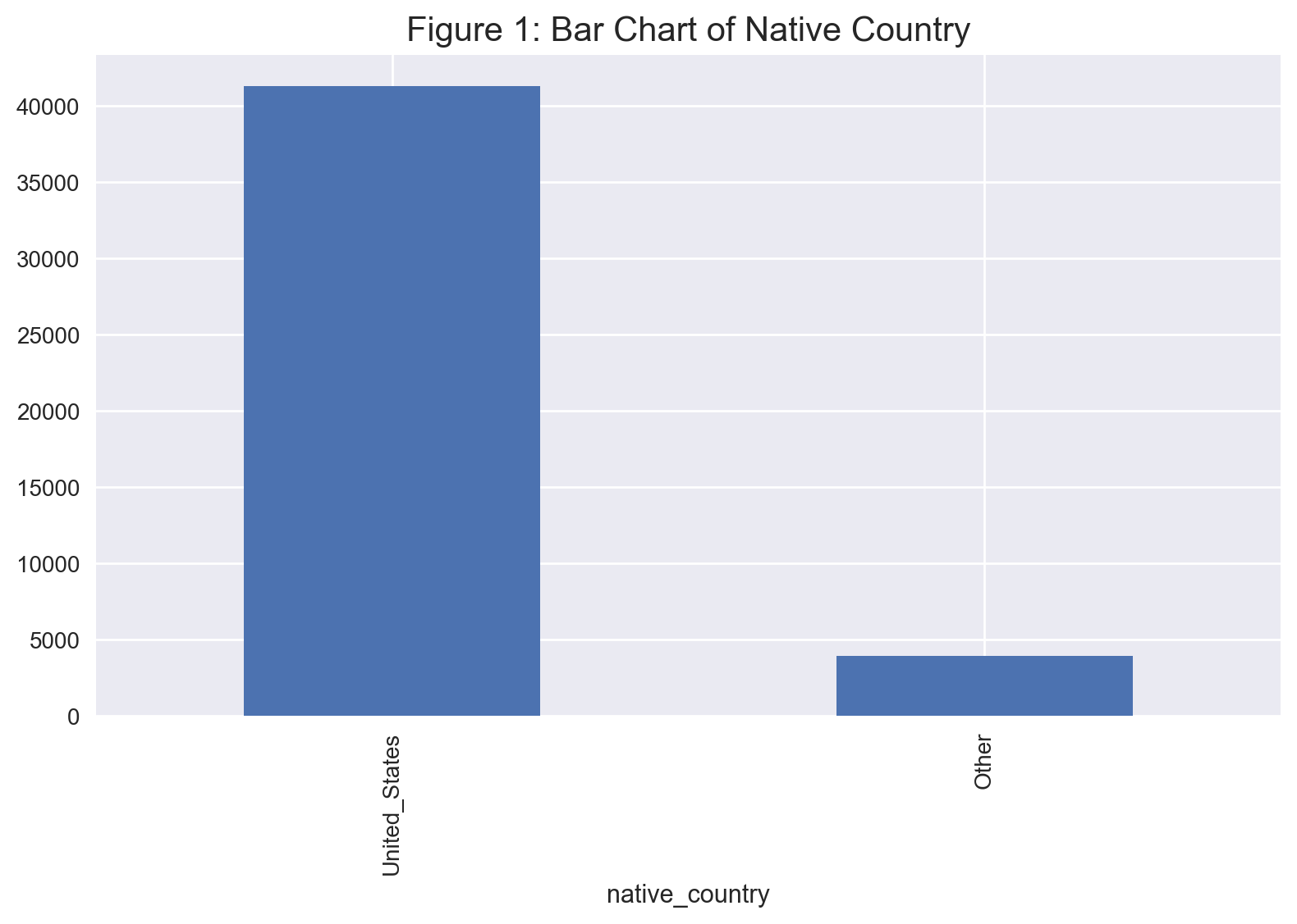
Since native-country is too granular and unbalanced, we group
countries as “Other” and “United_States”. Likewise, we also categorize
races as “Other” and “White”.
data.loc[data['native_country'] != 'United_States', 'native_country'] = 'Other'
data.loc[data['race'] != 'White', 'race'] = 'Other'
TIP 1: As a general comment, sometimes numerical features in a
dataset actually represent categorical features. As an example, suppose
each state of Australia is encoded as an integer between 1 and 8, say as
StateID column in a dataframe called df. This would still be a
categorical variable. For your code to work correctly in such cases, you
need to change the data type of this column from numeric to string as
follows:
df['StateID'] = df['StateID'].astype(str)
TIP 2: If you have a string column, say named col, that is
actually real-valued, you can change its data type as follows:
df['col'] = df['col'].astype(float)
Dependent Variable#
We need to correct the levels of the income categorical feature, which
is our dependent variable, to make sure it is binary.
print('Before correction, the number of unique income labels are: ')
print(data['income'].value_counts())
print("")

data['income'] = data['income'].str.rstrip(".")

print('After removing the dot, the number of unique income labels are: ')
print(data['income'].value_counts())
print("")
Before correction, the number of unique income labels are:
income
<=50K     22654
<=50K.    11360
>50K       7508
>50K.      3700
Name: count, dtype: int64

After removing the dot, the number of unique income labels are:
income
<=50K    34014
>50K     11208
Name: count, dtype: int64
WARNING: The Statsmodels module does not play nice when you have
mathematical symbols such as “-”, “+”, “<” and “>” in levels of
categorical variables (try it and you will get a syntax error). For this
reason, we will re-code income as low and high as below using the
replace() function in Pandas.
data['income'] = data['income'].replace({'<=50K': 'low', '>50K': 'high'})
data['income'].value_counts()
income
low     34014
high    11208
Name: count, dtype: int64
Data Exploration#
Our dataset can now be considered “clean” and ready for visualisation and statistical modeling.
Univariate Visualisation#
ax = data['native_country'].value_counts().plot(kind = 'bar')
ax.set_xticklabels(ax.get_xticklabels(), rotation = 90)
plt.tight_layout()
plt.title('Figure 1: Bar Chart of Native Country', fontsize = 15)
plt.show();
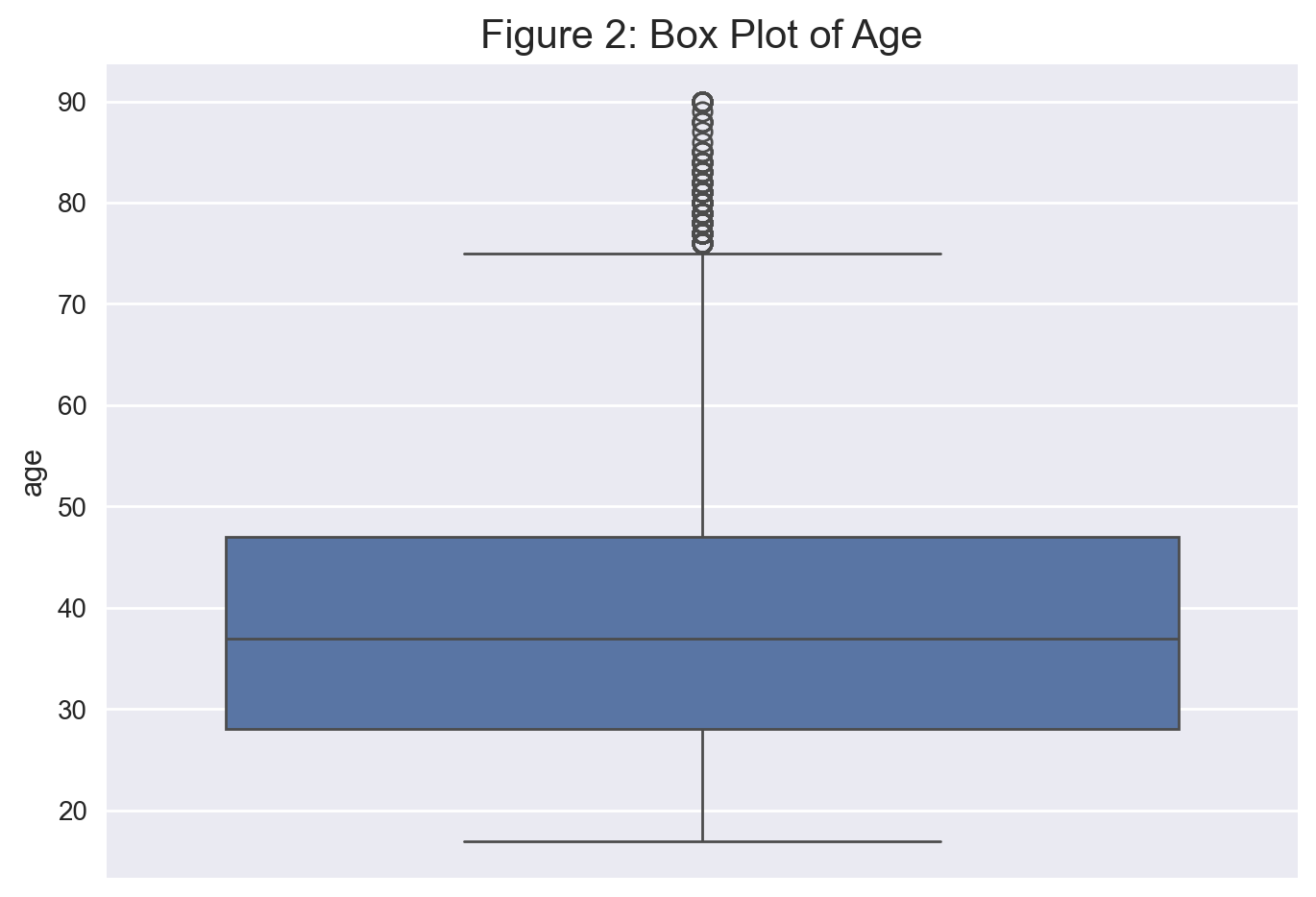
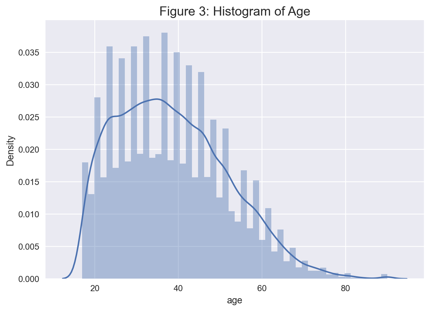
Let’s display a boxplot and histogram for age. Figure 2 shows that
this variable is right-skewed.
# get a box plot of age
sns.boxplot(data['age']).set_title('Figure 2: Box Plot of Age', fontsize = 15)
plt.show();
# get a histogram of age with kernel density estimate
sns.distplot(data['age'], kde = True).set_title('Figure 3: Histogram of Age', fontsize = 15)
plt.show();
Multivariate Visualisation#
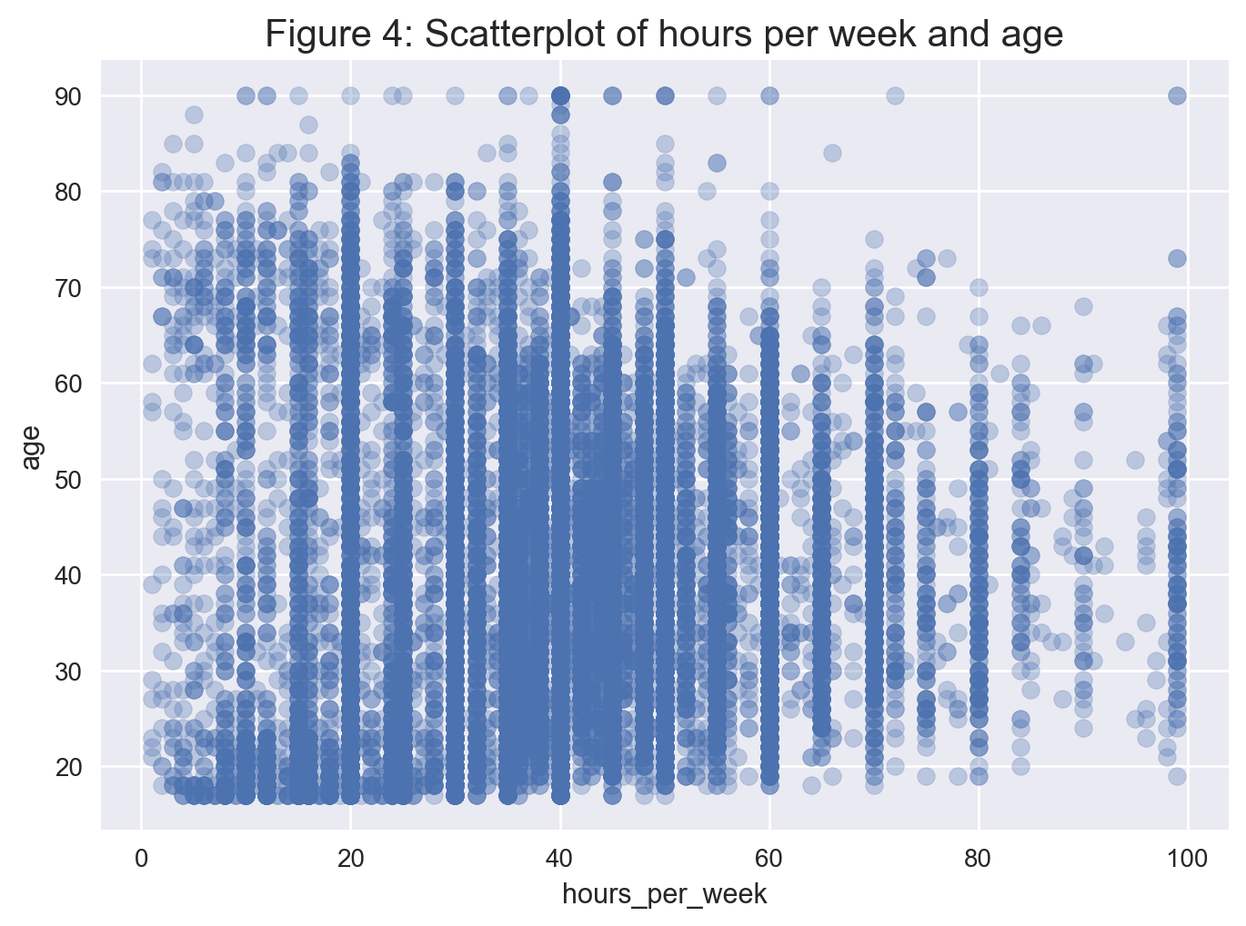
Scatterplot of Numeric Features and Age#
The scatterplot in Figure 4 shows no clear correlation between the age and hours_per_week numeric variables.
# store the values of hours-per-week
hpw = data['hours_per_week']

# get a scatter plot
plt.scatter(hpw, data['age'], alpha = 0.3)
plt.title('Figure 4: Scatterplot of hours per week and age', fontsize = 15)
plt.xlabel('hours_per_week')
plt.ylabel('age')
plt.show();
Categorical Attributes by Age#
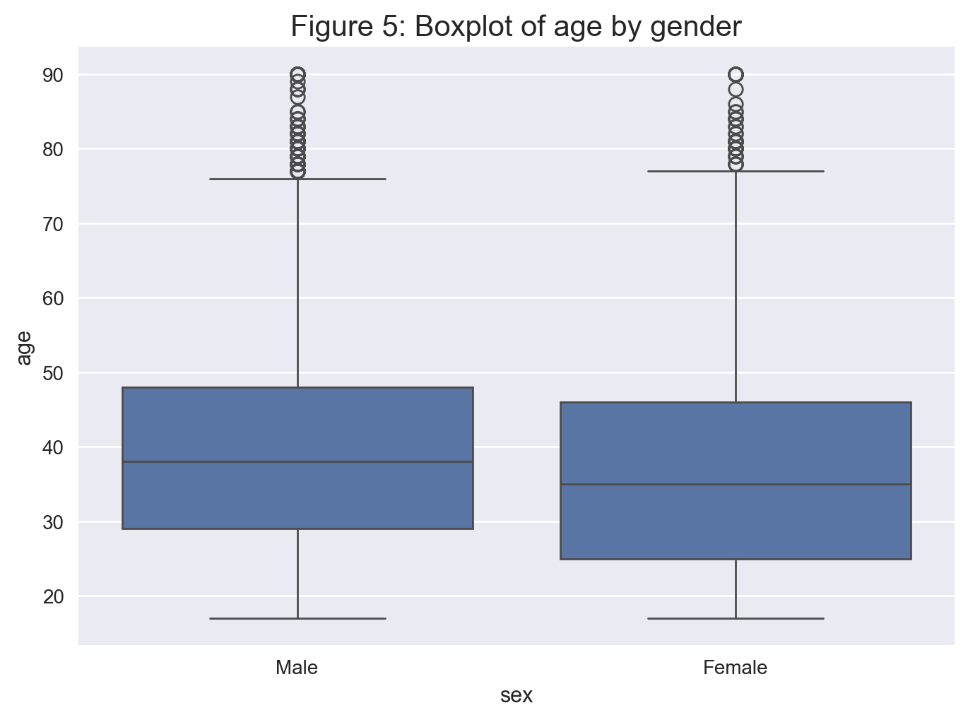
We can see that the distribution of age between each gender is similar.
# Creating a boxplot
sns.boxplot(x='sex', y='age', data=data);
plt.title('Figure 5: Boxplot of age by gender', fontsize = 15)
plt.show();
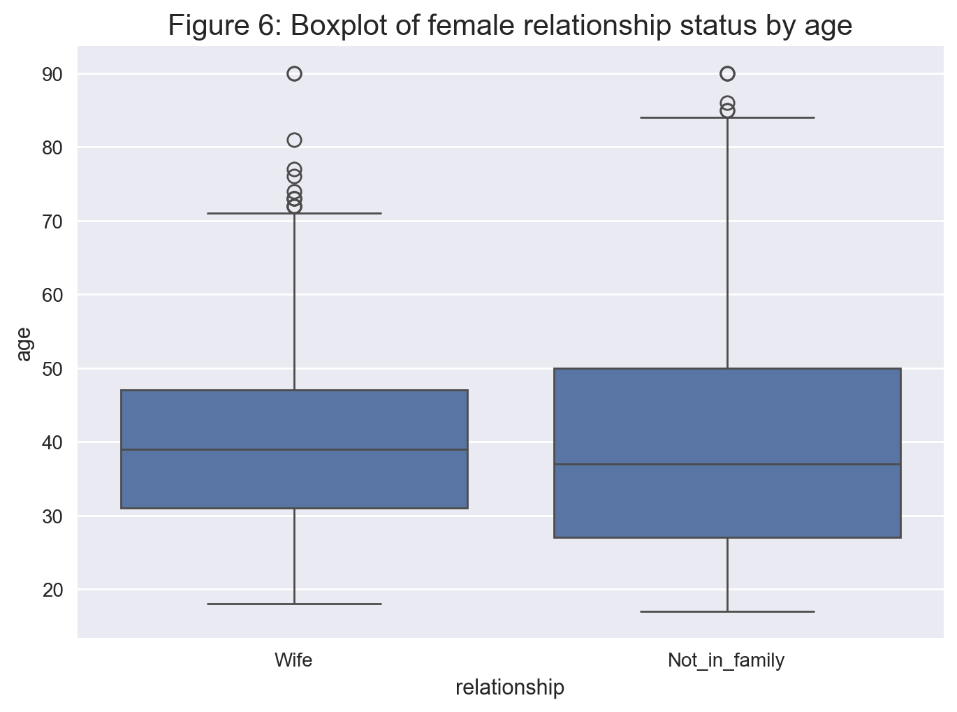
The distribution of married women and single women differ but have a similar median as seen in Figure 6. The whiskers suggest that women above the age of 70 are more likely to be single.
# Storing a list of booleans corresponding to whether the person is female and a wife or Not_in_family
family_female_mask = (data['relationship'].isin(['Not_in_family','Wife'])) & (data['sex'].isin(['Female']))

# Using the list of booleans previously found to select the index of rows
family_female = data[family_female_mask]

# Creating the boxplot
sns.boxplot(x='relationship', y='age', data=family_female);
plt.title('Figure 6: Boxplot of female relationship status by age', fontsize = 15)
plt.show();
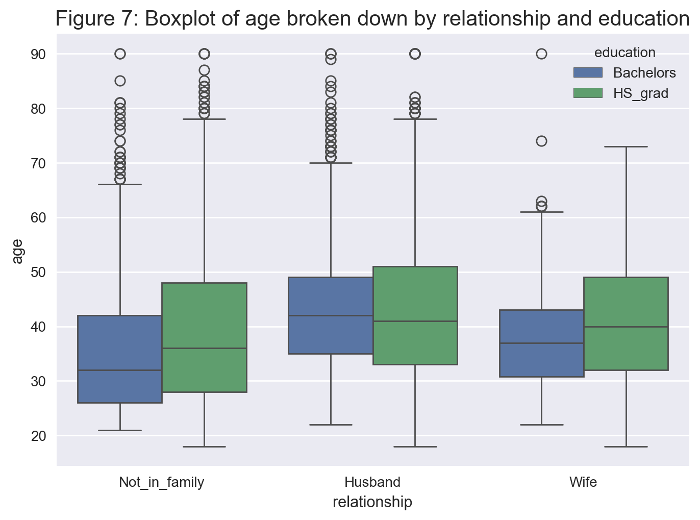
Facet plots#
From Figure 7, we see that generally the distribution of male bachelors and high school graduates is somewhat comparable within each relationship level.
# Getting the index of those who have completed their Bachelors or HS graduate
edu_mask = data['education'].isin(['Bachelors','HS_grad'])

# Getting the index of those who are male and Not_in_family or a Husband
family_male_mask = (data['relationship'].isin(['Not_in_family','Husband'])) & (data['sex'].isin(['Male']))

# Selecting the rows of those who are Not_in_family, husband or wife and
# have completed either a Bachelors or just graduated high school
education_relationship = data[(edu_mask & family_female_mask) | (edu_mask & family_male_mask)]

# Creating the boxplot
sns.boxplot(x='relationship', y='age', hue='education', data=education_relationship);
plt.title('Figure 7: Boxplot of age broken down by relationship and education', fontsize = 15)
plt.show();
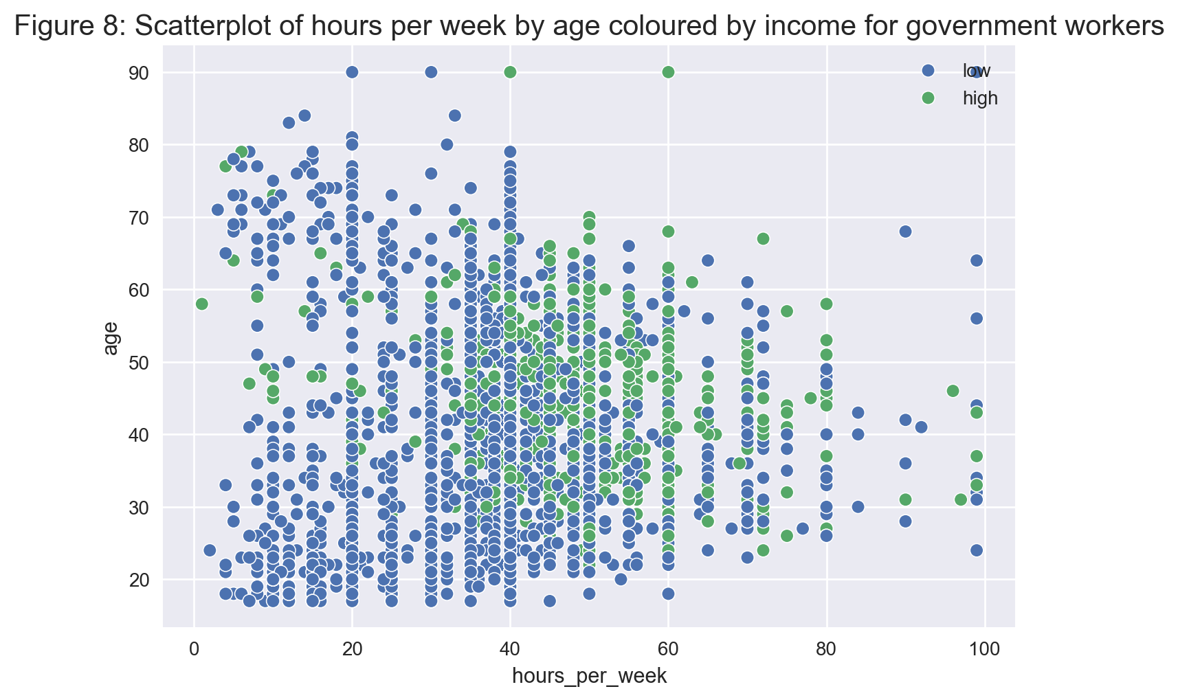
Although there is no clear overall pattern, we observe in Figure 8 that no government worker under the age of 40 earns over \$50k a year unless they work more than 20 hours a week.
# Getting the index of those who work in the government
gov_mask = data['workclass'].isin(['Federal_gov','Local_gov','State_gov'])

# creating a dataframe of those who work in the government
gov = data[gov_mask]

# creating a scatterplot
sns.scatterplot(x='hours_per_week', y='age', hue='income', data=gov)
plt.title('Figure 8: Scatterplot of hours per week by age coloured by income for government workers', fontsize = 15);
plt.legend(loc = 'upper right')
plt.show();
Statistical Modeling and Performance Evaluation#
Full Model#
We begin by fitting a multiple linear regression that predicts age
using all of the available features. We call this the full model. First
let’s take a quick peak at the clean data.
data.head()
| age | workclass | education | marital_status | occupation | relationship | race | sex | hours_per_week | native_country | income | capital | |
|---|---|---|---|---|---|---|---|---|---|---|---|---|
| 0 | 39 | State_gov | Bachelors | Never_married | Adm_clerical | Not_in_family | White | Male | 40 | United_States | low | 2174 |
| 1 | 50 | Self_emp_not_inc | Bachelors | Married_civ_spouse | Exec_managerial | Husband | White | Male | 13 | United_States | low | 0 |
| 2 | 38 | Private | HS_grad | Divorced | Handlers_cleaners | Not_in_family | White | Male | 40 | United_States | low | 0 |
| 3 | 53 | Private | 11th | Married_civ_spouse | Handlers_cleaners | Husband | Other | Male | 40 | United_States | low | 0 |
| 4 | 28 | Private | Bachelors | Married_civ_spouse | Prof_specialty | Wife | Other | Female | 40 | Other | low | 0 |
When constructing the regression formula, we can manually add all the independent features. On the other hand, if there are lots of independent variables, we can get smart and use some string function tricks as below.
# short and sweet
formula_string_indep_vars = ' + '.join(data.drop(columns='age').columns)
formula_string = 'age ~ ' + formula_string_indep_vars
print('formula_string: ', formula_string)
formula_string: age ~ workclass + education + marital_status + occupation + relationship + race + sex + hours_per_week + native_country + income + capital
The formula string above works just fine with the Statsmodels module.
The problem, however, is that we cannot do automatic variable selection
with this formula. What we need for this purpose is “one-hot-encoding”
of categorical features. For more information on this encoding, please
refer to this
page.
In the code chunk below, we first use the get_dummies() function in
Pandas for one-hot-encoding of categorical features and then we
construct a new formula string with the encoded features.
# one-hot-encoding of categorical features
# for this to work correctly, variable data types (numeric or categorical)
# must be correctly specified within the Pandas dataframe
data_encoded = pd.get_dummies(data, drop_first=True)
data_encoded.head()
| age | hours_per_week | capital | workclass_Local_gov | workclass_Private | workclass_Self_emp_inc | workclass_Self_emp_not_inc | workclass_State_gov | workclass_Without_pay | education_11th | ... | occupation_Transport_moving | relationship_Not_in_family | relationship_Other_relative | relationship_Own_child | relationship_Unmarried | relationship_Wife | race_White | sex_Male | native_country_United_States | income_low | |
|---|---|---|---|---|---|---|---|---|---|---|---|---|---|---|---|---|---|---|---|---|---|
| 0 | 39 | 40 | 2174 | False | False | False | False | True | False | False | ... | False | True | False | False | False | False | True | True | True | True |
| 1 | 50 | 13 | 0 | False | False | False | True | False | False | False | ... | False | False | False | False | False | False | True | True | True | True |
| 2 | 38 | 40 | 0 | False | True | False | False | False | False | False | ... | False | True | False | False | False | False | True | True | True | True |
| 3 | 53 | 40 | 0 | False | True | False | False | False | False | True | ... | False | False | False | False | False | False | False | True | True | True |
| 4 | 28 | 40 | 0 | False | True | False | False | False | False | False | ... | False | False | False | False | False | True | False | False | False | True |
5 rows × 52 columns
formula_string_indep_vars_encoded = ' + '.join(data_encoded.drop(columns='age').columns)
formula_string_encoded = 'age ~ ' + formula_string_indep_vars_encoded
print('formula_string_encoded: ', formula_string_encoded)
formula_string_encoded: age ~ hours_per_week + capital + workclass_Local_gov + workclass_Private + workclass_Self_emp_inc + workclass_Self_emp_not_inc + workclass_State_gov + workclass_Without_pay + education_11th + education_12th + education_1st_4th + education_5th_6th + education_7th_8th + education_9th + education_Assoc_acdm + education_Assoc_voc + education_Bachelors + education_Doctorate + education_HS_grad + education_Masters + education_Preschool + education_Prof_school + education_Some_college + marital_status_Married_AF_spouse + marital_status_Married_civ_spouse + marital_status_Married_spouse_absent + marital_status_Never_married + marital_status_Separated + marital_status_Widowed + occupation_Armed_Forces + occupation_Craft_repair + occupation_Exec_managerial + occupation_Farming_fishing + occupation_Handlers_cleaners + occupation_Machine_op_inspct + occupation_Other_service + occupation_Priv_house_serv + occupation_Prof_specialty + occupation_Protective_serv + occupation_Sales + occupation_Tech_support + occupation_Transport_moving + relationship_Not_in_family + relationship_Other_relative + relationship_Own_child + relationship_Unmarried + relationship_Wife + race_White + sex_Male + native_country_United_States + income_low
For fun, let’s add two interaction terms to our full model. Let’s add
the interaction of the capital feature with hours_per_week and
race_White respectively.
formula_string_encoded = formula_string_encoded + ' + hours_per_week:capital + race_White:capital'
Also, let’s add the square of the hours_per_week feature to illustrate
how we can add higher order terms to our linear regression.
formula_string_encoded = formula_string_encoded + ' + np.power(hours_per_week, 2)'
print('formula_string_encoded: ', formula_string_encoded)
formula_string_encoded: age ~ hours_per_week + capital + workclass_Local_gov + workclass_Private + workclass_Self_emp_inc + workclass_Self_emp_not_inc + workclass_State_gov + workclass_Without_pay + education_11th + education_12th + education_1st_4th + education_5th_6th + education_7th_8th + education_9th + education_Assoc_acdm + education_Assoc_voc + education_Bachelors + education_Doctorate + education_HS_grad + education_Masters + education_Preschool + education_Prof_school + education_Some_college + marital_status_Married_AF_spouse + marital_status_Married_civ_spouse + marital_status_Married_spouse_absent + marital_status_Never_married + marital_status_Separated + marital_status_Widowed + occupation_Armed_Forces + occupation_Craft_repair + occupation_Exec_managerial + occupation_Farming_fishing + occupation_Handlers_cleaners + occupation_Machine_op_inspct + occupation_Other_service + occupation_Priv_house_serv + occupation_Prof_specialty + occupation_Protective_serv + occupation_Sales + occupation_Tech_support + occupation_Transport_moving + relationship_Not_in_family + relationship_Other_relative + relationship_Own_child + relationship_Unmarried + relationship_Wife + race_White + sex_Male + native_country_United_States + income_low + hours_per_week:capital + race_White:capital + np.power(hours_per_week, 2)
Now that we have defined our statistical model formula as a Python string, we fit an OLS (ordinary least squares) model to our encoded data.
model_full = sm.formula.ols(formula=formula_string_encoded, data=data_encoded)
###
model_full_fitted = model_full.fit()
###
print(model_full_fitted.summary())
                            OLS Regression Results
==============================================================================
Dep. Variable:                    age   R-squared:                       0.406
Model:                            OLS   Adj. R-squared:                  0.405
Method:                 Least Squares   F-statistic:                     571.3
Date:                Tue, 23 Jul 2024   Prob (F-statistic):               0.00
Time:                        00:54:41   Log-Likelihood:            -1.6914e+05
No. Observations:               45222   AIC:                         3.384e+05
Df Residuals:                   45167   BIC:                         3.389e+05
Df Model:                          54
Covariance Type:            nonrobust
================================================================================================================
                                                   coef    std err          t      P>|t|      [0.025      0.975]
----------------------------------------------------------------------------------------------------------------
Intercept                                       58.8565      0.845     69.635      0.000      57.200      60.513
workclass_Local_gov[T.True]                     -0.5831      0.336     -1.737      0.082      -1.241       0.075
workclass_Private[T.True]                       -3.1473      0.285    -11.057      0.000      -3.705      -2.589
workclass_Self_emp_inc[T.True]                   1.5929      0.381      4.183      0.000       0.847       2.339
workclass_Self_emp_not_inc[T.True]               1.8802      0.331      5.675      0.000       1.231       2.530
workclass_State_gov[T.True]                     -1.9111      0.362     -5.284      0.000      -2.620      -1.202
workclass_Without_pay[T.True]                    7.5036      2.247      3.340      0.001       3.100      11.908
education_11th[T.True]                          -3.2940      0.387     -8.509      0.000      -4.053      -2.535
education_12th[T.True]                          -2.4467      0.516     -4.744      0.000      -3.458      -1.436
education_1st_4th[T.True]                        5.2143      0.756      6.897      0.000       3.732       6.696
education_5th_6th[T.True]                        4.0178      0.575      6.983      0.000       2.890       5.146
education_7th_8th[T.True]                        6.8474      0.462     14.827      0.000       5.942       7.753
education_9th[T.True]                            1.5526      0.490      3.170      0.002       0.593       2.512
education_Assoc_acdm[T.True]                    -2.0829      0.399     -5.226      0.000      -2.864      -1.302
education_Assoc_voc[T.True]                     -1.8617      0.377     -4.941      0.000      -2.600      -1.123
education_Bachelors[T.True]                     -1.5288      0.329     -4.643      0.000      -2.174      -0.883
education_Doctorate[T.True]                      3.3921      0.554      6.118      0.000       2.305       4.479
education_HS_grad[T.True]                       -0.6005      0.305     -1.968      0.049      -1.199      -0.003
education_Masters[T.True]                        1.2709      0.379      3.349      0.001       0.527       2.015
education_Preschool[T.True]                      4.8391      1.244      3.891      0.000       2.401       7.277
education_Prof_school[T.True]                    0.4821      0.503      0.958      0.338      -0.504       1.468
education_Some_college[T.True]                  -2.1039      0.313     -6.717      0.000      -2.718      -1.490
marital_status_Married_AF_spouse[T.True]       -15.3973      1.896     -8.121      0.000     -19.114     -11.681
marital_status_Married_civ_spouse[T.True]       -6.1876      0.605    -10.225      0.000      -7.374      -5.002
marital_status_Married_spouse_absent[T.True]    -2.5870      0.457     -5.667      0.000      -3.482      -1.692
marital_status_Never_married[T.True]           -11.9959      0.170    -70.591      0.000     -12.329     -11.663
marital_status_Separated[T.True]                -2.9265      0.302     -9.687      0.000      -3.519      -2.334
marital_status_Widowed[T.True]                  13.5010      0.318     42.520      0.000      12.879      14.123
occupation_Armed_Forces[T.True]                 -6.4631      2.742     -2.357      0.018     -11.838      -1.089
occupation_Craft_repair[T.True]                 -1.4627      0.208     -7.025      0.000      -1.871      -1.055
occupation_Exec_managerial[T.True]               0.5189      0.204      2.544      0.011       0.119       0.919
occupation_Farming_fishing[T.True]              -0.0065      0.322     -0.020      0.984      -0.638       0.625
occupation_Handlers_cleaners[T.True]            -2.6262      0.277     -9.466      0.000      -3.170      -2.082
occupation_Machine_op_inspct[T.True]            -1.2234      0.244     -5.024      0.000      -1.701      -0.746
occupation_Other_service[T.True]                -1.4299      0.207     -6.895      0.000      -1.836      -1.023
occupation_Priv_house_serv[T.True]               3.0495      0.692      4.406      0.000       1.693       4.406
occupation_Prof_specialty[T.True]               -0.7470      0.216     -3.459      0.001      -1.170      -0.324
occupation_Protective_serv[T.True]              -1.7801      0.371     -4.800      0.000      -2.507      -1.053
occupation_Sales[T.True]                        -0.8718      0.203     -4.288      0.000      -1.270      -0.473
occupation_Tech_support[T.True]                 -1.2322      0.307     -4.015      0.000      -1.834      -0.631
occupation_Transport_moving[T.True]              0.2230      0.268      0.832      0.406      -0.303       0.749
relationship_Not_in_family[T.True]              -4.0503      0.603     -6.716      0.000      -5.232      -2.868
relationship_Other_relative[T.True]             -6.8905      0.590    -11.689      0.000      -8.046      -5.735
relationship_Own_child[T.True]                 -11.9082      0.600    -19.862      0.000     -13.083     -10.733
relationship_Unmarried[T.True]                  -6.1890      0.624     -9.919      0.000      -7.412      -4.966
relationship_Wife[T.True]                       -3.9954      0.273    -14.611      0.000      -4.531      -3.459
race_White[T.True]                              -1.0056      0.145     -6.919      0.000      -1.290      -0.721
sex_Male[T.True]                                -0.1782      0.146     -1.223      0.221      -0.464       0.107
native_country_United_States[T.True]             1.4129      0.185      7.647      0.000       1.051       1.775
income_low[T.True]                              -2.4367      0.138    -17.616      0.000      -2.708      -2.166
hours_per_week                                  -0.1571      0.014    -11.106      0.000      -0.185      -0.129
capital                                          0.0001   3.22e-05      3.492      0.000    4.93e-05       0.000
race_White[T.True]:capital                    3.006e-05   2.12e-05      1.418      0.156   -1.15e-05    7.16e-05
hours_per_week:capital                       -2.148e-06   5.02e-07     -4.283      0.000   -3.13e-06   -1.17e-06
np.power(hours_per_week, 2)                      0.0010      0.000      6.350      0.000       0.001       0.001
==============================================================================
Omnibus:                     3966.388   Durbin-Watson:                   2.001
Prob(Omnibus):                  0.000   Jarque-Bera (JB):             5729.860
Skew:                           0.703   Prob(JB):                         0.00
Kurtosis:                       4.033   Cond. No.                     2.26e+07
==============================================================================

Notes:
[1] Standard Errors assume that the covariance matrix of the errors is correctly specified.
[2] The condition number is large, 2.26e+07. This might indicate that there are
strong multicollinearity or other numerical problems.
The full model has an adjusted R-squared value of 0.405, which means that only 40% of the variance is explained by the model. By looking at the p-values, we observe that the majority of them are highly significant, though there are a few insignificant variables at a 5% level.
Let’s define a new data frame for actual age vs. predicted age and the residuals for the full model. We will use this data frame when plotting predicted values and the regression residuals.
residuals_full = pd.DataFrame({'actual': data_encoded['age'],
                               'predicted': model_full_fitted.fittedvalues,
                               'residual': model_full_fitted.resid})
residuals_full.head(10)
| actual | predicted | residual | |
|---|---|---|---|
| 0 | 39 | 32.570133 | 6.429867 |
| 1 | 50 | 49.455511 | 0.544489 |
| 2 | 38 | 41.508711 | -3.508711 |
| 3 | 53 | 37.683573 | 15.316427 |
| 4 | 28 | 36.097893 | -8.097893 |
| 5 | 37 | 40.570690 | -3.570690 |
| 6 | 49 | 44.495664 | 4.504336 |
| 7 | 52 | 49.611524 | 2.388476 |
| 8 | 31 | 35.683539 | -4.683539 |
| 9 | 42 | 44.318118 | -2.318118 |
Let’s plot actual age values vs. predicted values.
def plot_line(axis, slope, intercept, **kargs):
    xmin, xmax = axis.get_xlim()
    plt.plot([xmin, xmax], [xmin*slope+intercept, xmax*slope+intercept], **kargs)

# Creating scatter plot
plt.scatter(residuals_full['actual'], residuals_full['predicted'], alpha=0.3);
plot_line(axis=plt.gca(), slope=1, intercept=0, c="red");
plt.xlabel('Actual Age');
plt.ylabel('Predicted Age');
plt.title('Figure 9: Scatter plot of actual vs. predicted age for the Full Model', fontsize=15);
plt.show();
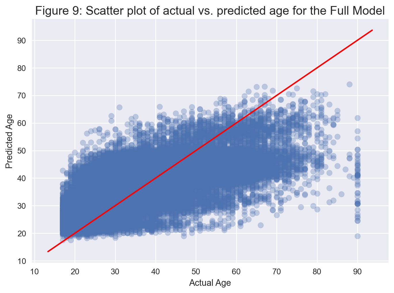
From Figure 9, we observe that the model never produces a prediction above 80 even though the oldest person in the dataset is 90.
We will now check the diagnostics for the full model.
Full Model Diagnostic Checks#
We would like to check whether there are indications of violations of the regression assumptions, which are
linearity of the relationship between target variable and the independent variables
constant variance of the errors
normality of the residual distribution
statistical independence of the residuals
Let’s first get a scatter plot of residuals (as a function of predicted
age).
plt.scatter(residuals_full['predicted'], residuals_full['residual'], alpha=0.3);
plt.xlabel('Predicted Age');
plt.ylabel('Residuals')
plt.title('Figure 10(a): Scatterplot of residuals vs. predicted age for Full Model', fontsize=15)
plt.show();
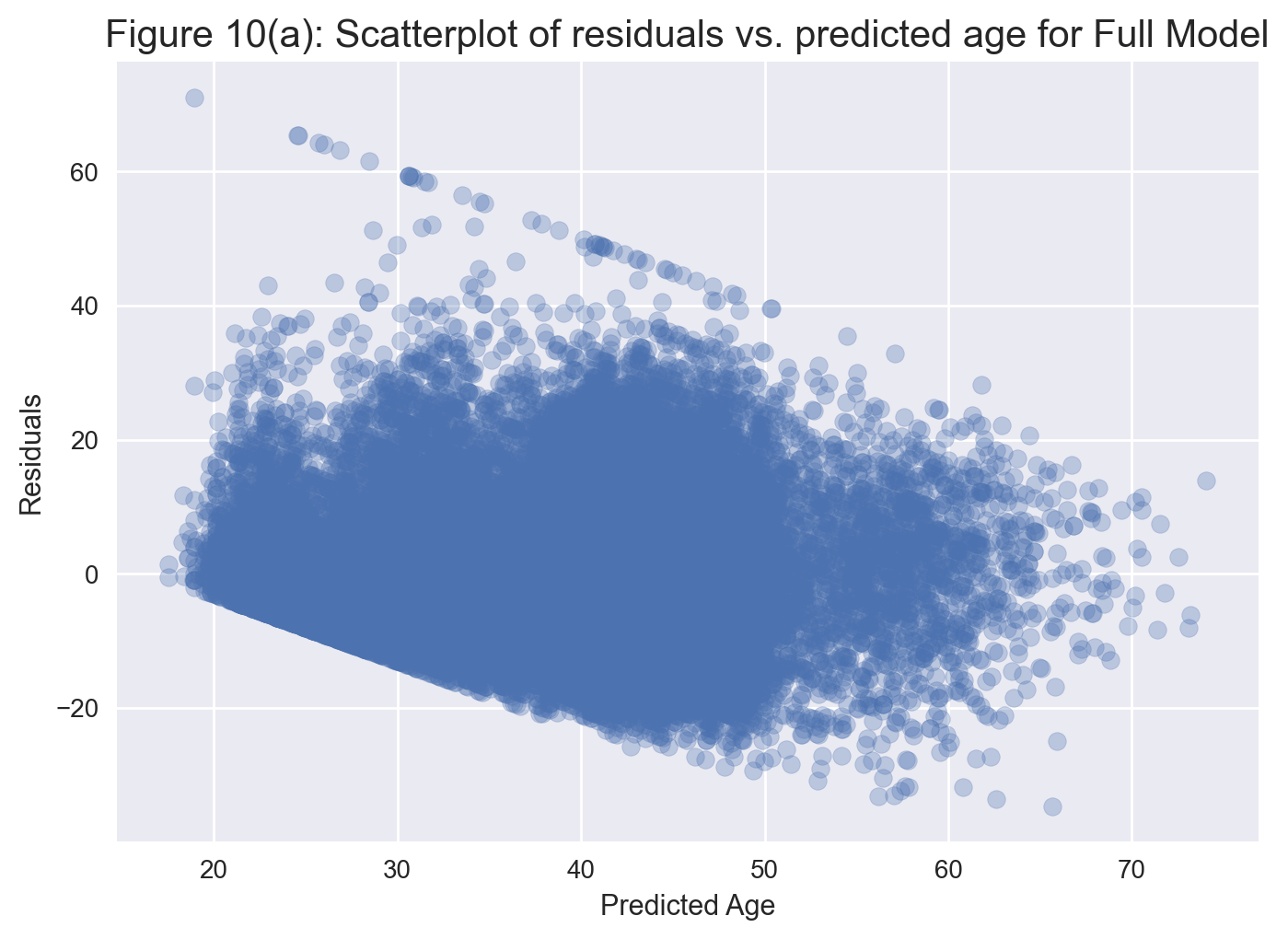
From Figure 10(a), we see that, rather than being mostly random and centered around 0, the residuals exhibit a banding pattern, especially when predicted age is below 50. This pattern indicates that the constant variability assumption of linear regression is not quite satisfied in this case.
Let’s now plot actual age vs. residuals.
plt.scatter(residuals_full['actual'], residuals_full['residual'], alpha=0.3);
plt.xlabel('Actual Age');
plt.ylabel('Residuals')
plt.title('Figure 10(b): Scatterplot of residuals vs. actual age for Full Model', fontsize=15)
plt.show();
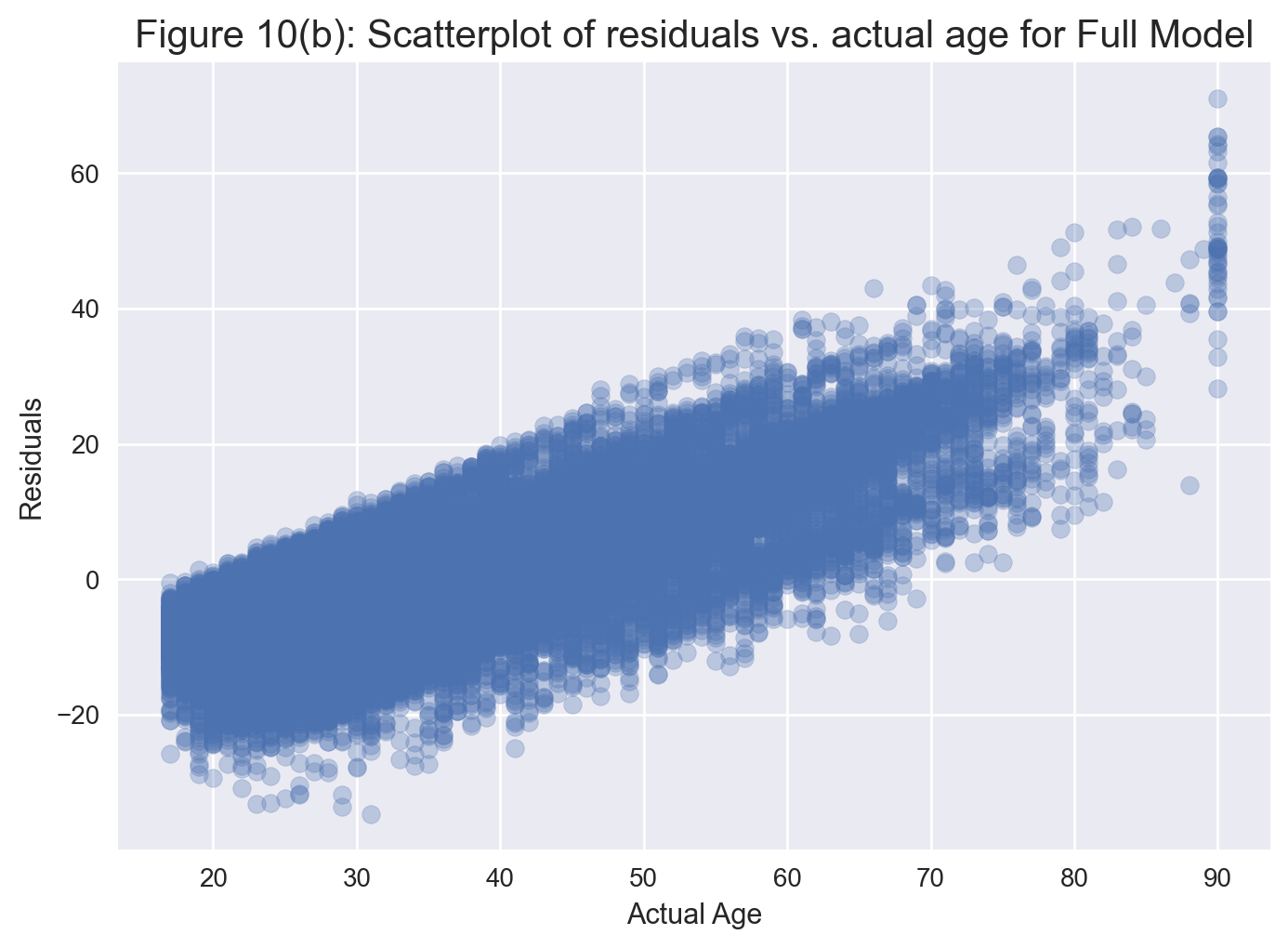
We notice that the model overestimates younger ages and underestimates older ages. In particular, for those younger than the age of 30, the model predicts much older ages. Also, for those above the age of 80, the model predicts significantly younger ages.
Let’s overlay the histograms of actual vs. predicted age on the same plot.
plt.hist(residuals_full['actual'], label='actual', bins=20, alpha=0.7);
plt.hist(residuals_full['predicted'], label='predicted', bins=20, alpha=0.7);
plt.xlabel('Age');
plt.ylabel('Frequency');
plt.title('Figure 11: Histograms of actual age vs. predicted age for Full Model', fontsize=15);
plt.legend()
plt.show();
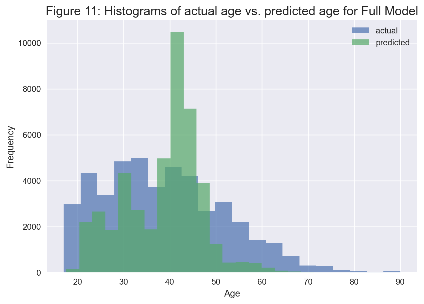
We notice that their distributions are quite different. In particular, the model’s predictions are highly clustered around mid-40’s.
Let’s now have look at the histogram of the residuals.
plt.hist(residuals_full['residual'], bins = 20);
plt.xlabel('Residual');
plt.ylabel('Frequency');
plt.title('Figure 12: Histogram of residuals for Full Model', fontsize=15);
plt.show();

From Figure 12, the histogram of residuals looks somewhat symmetric, though slightly right-skewed. Nonetheless, it seems the normality assumption of linear regression is not significantly violated in this particular case.
Backwards Feature Selection#
We now perform backwards feature selection using p-values. It appears
Statsmodels does not have any canned code for automatic feature
selection, so we wrote one ourselves.
formula_string_encoded
'age ~ hours_per_week + capital + workclass_Local_gov + workclass_Private + workclass_Self_emp_inc + workclass_Self_emp_not_inc + workclass_State_gov + workclass_Without_pay + education_11th + education_12th + education_1st_4th + education_5th_6th + education_7th_8th + education_9th + education_Assoc_acdm + education_Assoc_voc + education_Bachelors + education_Doctorate + education_HS_grad + education_Masters + education_Preschool + education_Prof_school + education_Some_college + marital_status_Married_AF_spouse + marital_status_Married_civ_spouse + marital_status_Married_spouse_absent + marital_status_Never_married + marital_status_Separated + marital_status_Widowed + occupation_Armed_Forces + occupation_Craft_repair + occupation_Exec_managerial + occupation_Farming_fishing + occupation_Handlers_cleaners + occupation_Machine_op_inspct + occupation_Other_service + occupation_Priv_house_serv + occupation_Prof_specialty + occupation_Protective_serv + occupation_Sales + occupation_Tech_support + occupation_Transport_moving + relationship_Not_in_family + relationship_Other_relative + relationship_Own_child + relationship_Unmarried + relationship_Wife + race_White + sex_Male + native_country_United_States + income_low + hours_per_week:capital + race_White:capital + np.power(hours_per_week, 2)'
import re

## create the patsy model description from formula
patsy_description = patsy.ModelDesc.from_formula(formula_string_encoded)

# initialize feature-selected fit to full model
linreg_fit = model_full_fitted

# do backwards elimination using p-values
p_val_cutoff = 0.05

## WARNING 1: The code below assumes that the Intercept term is present in the model.
## WARNING 2: It will work only with main effects and two-way interactions, if any.

print('\nPerforming backwards feature selection using p-values:')

while True:

    # uncomment the line below if you would like to see the regression summary
    # in each step:
    # ### print(linreg_fit.summary())

    pval_series = linreg_fit.pvalues.drop(labels='Intercept')
    pval_series = pval_series.sort_values(ascending=False)
    term = pval_series.index[0]
    pval = pval_series[0]
    if (pval < p_val_cutoff):
        break

    print(f'\nRemoving term "{term}" with p-value {pval:.4}')

    term_components = term.split(':')

    if (len(term_components) == 1): ## this is a main effect term

        term_to_remove = re.sub(r'\[.*?\]', '', term_components[0])

        patsy_description.rhs_termlist.remove(patsy.Term([patsy.EvalFactor(term_to_remove)]))


    else: ## this is an interaction term

        term_to_remove1 = re.sub(r'\[.*?\]', '', term_components[0])
        term_to_remove2 = re.sub(r'\[.*?\]', '', term_components[1])

        patsy_description.rhs_termlist.remove(patsy.Term([patsy.EvalFactor(term_to_remove1),
                                                          patsy.EvalFactor(term_to_remove2)]))

    linreg_fit = smf.ols(formula=patsy_description, data=data_encoded).fit()

#########
## this is the clean fit after backwards elimination
model_reduced_fitted = smf.ols(formula = patsy_description, data = data_encoded).fit()
#########

#########
print("\n***")
print(model_reduced_fitted.summary())
print("***")
print(f"Regression number of terms: {len(model_reduced_fitted.model.exog_names)}")
print(f"Regression F-distribution p-value: {model_reduced_fitted.f_pvalue:.4f}")
print(f"Regression R-squared: {model_reduced_fitted.rsquared:.4f}")
print(f"Regression Adjusted R-squared: {model_reduced_fitted.rsquared_adj:.4f}")
Performing backwards feature selection using p-values:

Removing term "occupation_Farming_fishing[T.True]" with p-value 0.984

Removing term "occupation_Transport_moving[T.True]" with p-value 0.3774

Removing term "education_Prof_school[T.True]" with p-value 0.3591

Removing term "sex_Male[T.True]" with p-value 0.2642

Removing term "race_White[T.True]:capital" with p-value 0.1615

Removing term "workclass_Local_gov[T.True]" with p-value 0.09358

***
                            OLS Regression Results
==============================================================================
Dep. Variable:                    age   R-squared:                       0.406
Model:                            OLS   Adj. R-squared:                  0.405
Method:                 Least Squares   F-statistic:                     642.5
Date:                Tue, 23 Jul 2024   Prob (F-statistic):               0.00
Time:                        00:54:44   Log-Likelihood:            -1.6914e+05
No. Observations:               45222   AIC:                         3.384e+05
Df Residuals:                   45173   BIC:                         3.388e+05
Df Model:                          48
Covariance Type:            nonrobust
================================================================================================================
                                                   coef    std err          t      P>|t|      [0.025      0.975]
----------------------------------------------------------------------------------------------------------------
Intercept                                       58.5679      0.790     74.140      0.000      57.020      60.116
workclass_Private[T.True]                       -2.7499      0.172    -15.951      0.000      -3.088      -2.412
workclass_Self_emp_inc[T.True]                   1.9866      0.307      6.477      0.000       1.385       2.588
workclass_Self_emp_not_inc[T.True]               2.2638      0.236      9.610      0.000       1.802       2.726
workclass_State_gov[T.True]                     -1.5082      0.278     -5.422      0.000      -2.053      -0.963
workclass_Without_pay[T.True]                    7.8647      2.233      3.522      0.000       3.488      12.242
education_11th[T.True]                          -3.4571      0.348     -9.931      0.000      -4.139      -2.775
education_12th[T.True]                          -2.6152      0.487     -5.373      0.000      -3.569      -1.661
education_1st_4th[T.True]                        5.0367      0.736      6.843      0.000       3.594       6.479
education_5th_6th[T.True]                        3.8423      0.549      6.994      0.000       2.766       4.919
education_7th_8th[T.True]                        6.6783      0.429     15.573      0.000       5.838       7.519
education_9th[T.True]                            1.3880      0.459      3.021      0.003       0.487       2.289
education_Assoc_acdm[T.True]                    -2.2605      0.352     -6.419      0.000      -2.951      -1.570
education_Assoc_voc[T.True]                     -2.0396      0.329     -6.208      0.000      -2.684      -1.396
education_Bachelors[T.True]                     -1.7276      0.262     -6.588      0.000      -2.242      -1.214
education_Doctorate[T.True]                      3.1805      0.503      6.321      0.000       2.194       4.167
education_HS_grad[T.True]                       -0.7660      0.250     -3.061      0.002      -1.257      -0.275
education_Masters[T.True]                        1.0459      0.314      3.326      0.001       0.430       1.662
education_Preschool[T.True]                      4.6321      1.231      3.764      0.000       2.220       7.044
education_Some_college[T.True]                  -2.2759      0.256     -8.882      0.000      -2.778      -1.774
marital_status_Married_AF_spouse[T.True]       -15.3512      1.896     -8.097      0.000     -19.067     -11.635
marital_status_Married_civ_spouse[T.True]       -6.2001      0.605    -10.247      0.000      -7.386      -5.014
marital_status_Married_spouse_absent[T.True]    -2.5991      0.456     -5.696      0.000      -3.494      -1.705
marital_status_Never_married[T.True]           -12.0107      0.169    -70.961      0.000     -12.342     -11.679
marital_status_Separated[T.True]                -2.9334      0.302     -9.711      0.000      -3.525      -2.341
marital_status_Widowed[T.True]                  13.5172      0.317     42.689      0.000      12.897      14.138
occupation_Armed_Forces[T.True]                 -6.1629      2.732     -2.256      0.024     -11.517      -0.808
occupation_Craft_repair[T.True]                 -1.5761      0.173     -9.121      0.000      -1.915      -1.237
occupation_Exec_managerial[T.True]               0.4658      0.180      2.581      0.010       0.112       0.819
occupation_Handlers_cleaners[T.True]            -2.7455      0.253    -10.860      0.000      -3.241      -2.250
occupation_Machine_op_inspct[T.True]            -1.3151      0.219     -6.001      0.000      -1.745      -0.886
occupation_Other_service[T.True]                -1.4980      0.185     -8.090      0.000      -1.861      -1.135
occupation_Priv_house_serv[T.True]               3.0454      0.686      4.443      0.000       1.702       4.389
occupation_Prof_specialty[T.True]               -0.7794      0.191     -4.078      0.000      -1.154      -0.405
occupation_Protective_serv[T.True]              -1.9512      0.353     -5.527      0.000      -2.643      -1.259
occupation_Sales[T.True]                        -0.9336      0.179     -5.223      0.000      -1.284      -0.583
occupation_Tech_support[T.True]                 -1.2731      0.294     -4.331      0.000      -1.849      -0.697
relationship_Not_in_family[T.True]              -3.9907      0.601     -6.645      0.000      -5.168      -2.814
relationship_Other_relative[T.True]             -6.8363      0.587    -11.650      0.000      -7.986      -5.686
relationship_Own_child[T.True]                 -11.8623      0.597    -19.867      0.000     -13.033     -10.692
relationship_Unmarried[T.True]                  -6.0981      0.618     -9.875      0.000      -7.308      -4.888
relationship_Wife[T.True]                       -3.8670      0.240    -16.083      0.000      -4.338      -3.396
race_White[T.True]                              -0.9984      0.144     -6.919      0.000      -1.281      -0.716
native_country_United_States[T.True]             1.4226      0.185      7.708      0.000       1.061       1.784
income_low[T.True]                              -2.4513      0.137    -17.895      0.000      -2.720      -2.183
hours_per_week                                  -0.1575      0.014    -11.164      0.000      -0.185      -0.130
capital                                          0.0001    2.6e-05      5.345      0.000    8.81e-05       0.000
hours_per_week:capital                        -2.13e-06   5.01e-07     -4.247      0.000   -3.11e-06   -1.15e-06
np.power(hours_per_week, 2)                      0.0010      0.000      6.379      0.000       0.001       0.001
==============================================================================
Omnibus:                     3959.253   Durbin-Watson:                   2.001
Prob(Omnibus):                  0.000   Jarque-Bera (JB):             5717.587
Skew:                           0.702   Prob(JB):                         0.00
Kurtosis:                       4.032   Cond. No.                     2.25e+07
==============================================================================

Notes:
[1] Standard Errors assume that the covariance matrix of the errors is correctly specified.
[2] The condition number is large, 2.25e+07. This might indicate that there are
strong multicollinearity or other numerical problems.
***
Regression number of terms: 49
Regression F-distribution p-value: 0.0000
Regression R-squared: 0.4057
Regression Adjusted R-squared: 0.4051
Similar to what we did for the full model, let’s define a new data frame for actual age vs. predicted age and the residuals for the reduced model.
residuals_reduced = pd.DataFrame({'actual': data_encoded['age'],
                                  'predicted': model_reduced_fitted.fittedvalues,
                                  'residual': model_reduced_fitted.resid})
residuals_reduced.head(10)
| actual | predicted | residual | |
|---|---|---|---|
| 0 | 39 | 32.690335 | 6.309665 |
| 1 | 50 | 49.461020 | 0.538980 |
| 2 | 38 | 41.558042 | -3.558042 |
| 3 | 53 | 37.655981 | 15.344019 |
| 4 | 28 | 36.062133 | -8.062133 |
| 5 | 37 | 40.504922 | -3.504922 |
| 6 | 49 | 44.397983 | 4.602017 |
| 7 | 52 | 49.654315 | 2.345685 |
| 8 | 31 | 35.544969 | -4.544969 |
| 9 | 42 | 44.329267 | -2.329267 |
# get a scatter plot
plt.scatter(residuals_reduced['actual'], residuals_reduced['predicted'], alpha=0.3);
plot_line(axis=plt.gca(), slope=1, intercept=0, c="red");
plt.xlabel('Age');
plt.ylabel('Predicted Age');
plt.title('Figure 13: Scatter plot of actual vs. predicted age for Reduced Model', fontsize=15);
plt.show();
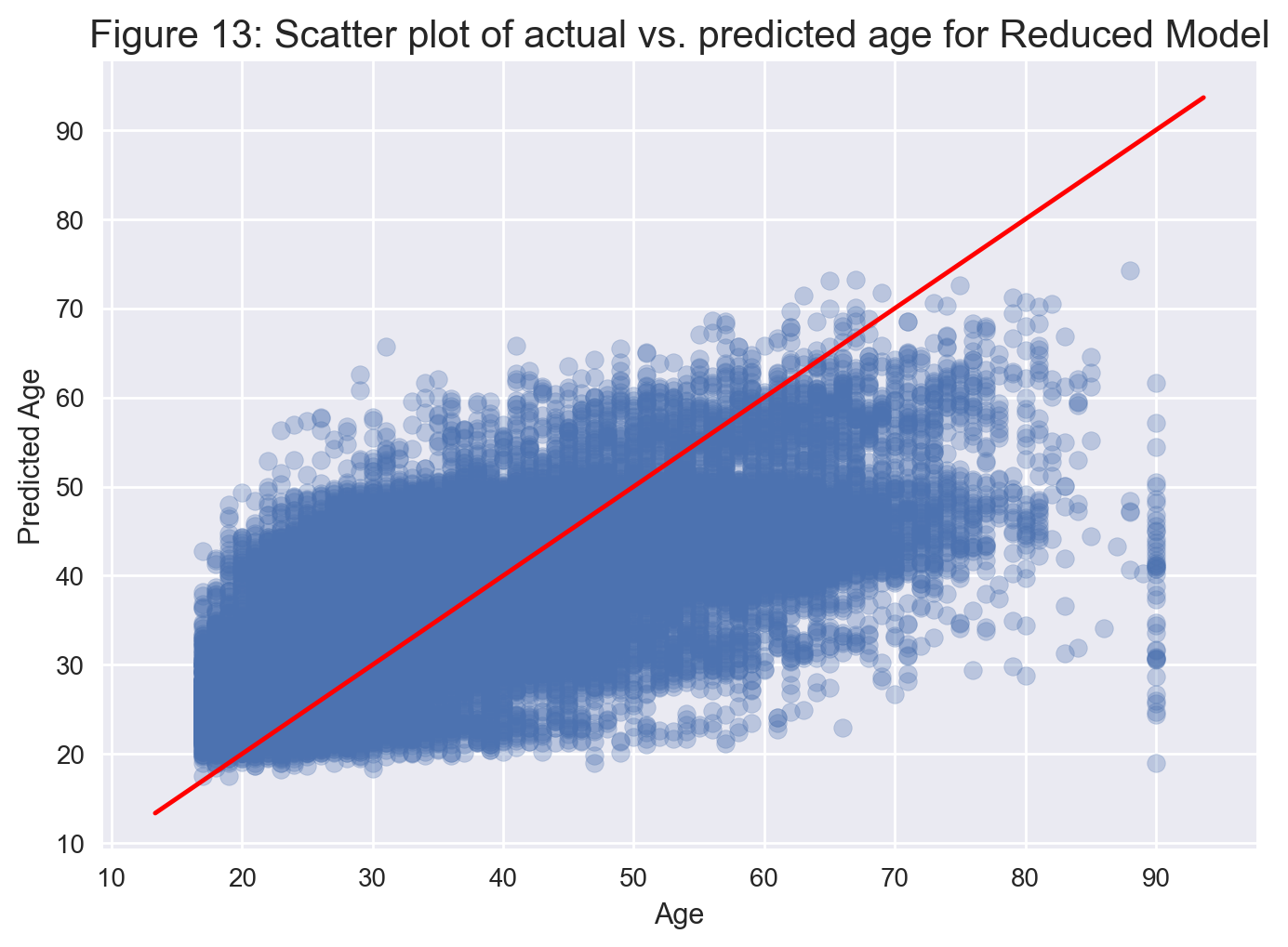
This model returns an Adjusted R-squared of 0.404, meaning the reduced model still explains about 40% of the variance, but with 6 less variables. Looking at the p-values, they are all significant at the 5% level, as expected. From Figure 13, we still have the same issues with our model. That is, the model overestimates younger ages and underestimates older ages. We will now perform the diagnostic checks on this reduced model.
Reduced Model Diagnostic Checks#
Let’s first get a scatter plot of residuals (as a function of predicted age).
plt.scatter(residuals_reduced['predicted'], residuals_reduced['residual'], alpha=0.3);
plt.xlabel('Predicted Age');
plt.ylabel('Residuals')
plt.title('Figure 14: Scatter plot of residuals vs. predicted age for Reduced Model', fontsize=15)
plt.show();
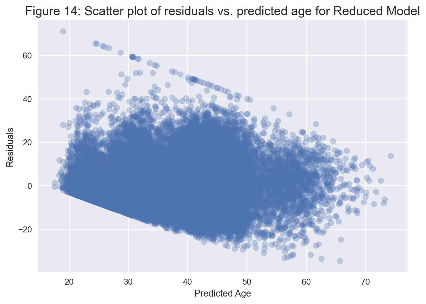
Figure 14 looks very similar to Figure 10(a), suggesting that the residuals exhibit the same banding pattern.
Let’s now have look at the histogram of the residuals for the reduced model.
plt.hist(residuals_reduced['residual'], bins = 20);
plt.xlabel('Residual');
plt.ylabel('Frequency');
plt.title('Figure 15: Histogram of residuals for Reduced Model', fontsize = 15)
plt.show();
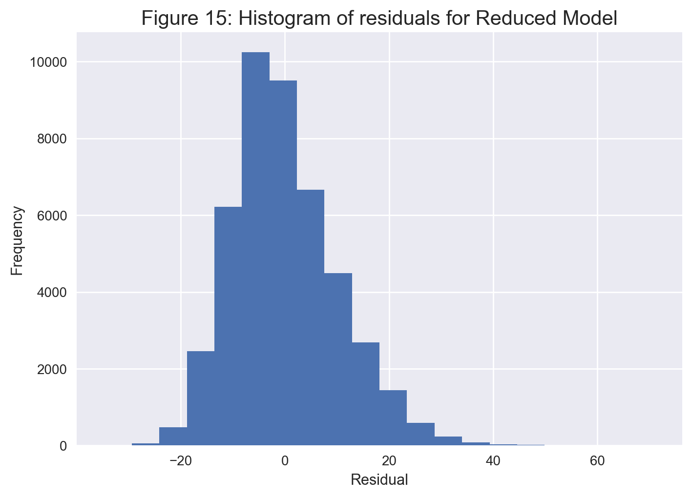
From Figure 15, there is again a somewhat symmetric histogram around zero, which suggests that the residuals are somewhat normally distributed.
Summary and Conclusions#
Using our independent variables, we were able to get a full model with an Adjusted R-squared value of about 40%. After backwards variable selection with a p-value cutoff value of 0.05, we were able to maintain the same performance but with 6 less variables. Our final model has 49 variables all together with a model p-value of 0.
Diagnostic checks with residual scatter plots indicate that, rather than being random and centered around 0, the residuals exhibit a banding pattern, especially when predicted age is below 50. This pattern indicates that the constant variability assumption of linear regression is not quite satisfied in this case. On the other hand, residual histograms suggest that there are no significant violations of the normality assumption on the residuals.
The final multiple linear regression model has an Adjusted R-squared value of about 40%, which is pretty low. So, it appears that the variables we used are not quite adequate for accurately predicting the age of an individual in the 1994 US Census dataset within a multiple linear regression framework. A good next step might involve adding some more interaction terms and maybe some other higher order terms to see if this would result in some improvement for the Adjusted R-squared value. Nonetheless, it might be the case that nonlinear models such as a neural network might be more appropriate for the task at hand rather than a linear regression model.
Our regression model appears to predict age correctly within $\pm40$ years in general, though this is clearly a huge margin of error for the model to be useful for any practical purposes. Furthermore, our model has some rather significant issues. Specifically, our model consistently overestimates younger ages and underestimates older ages. In particular, for those younger than the age of 30, the model predicts much older ages. Also, for those above the age of 80, the model predicts significantly younger ages.
References#
Lichman, M. (2013). UCI Machine Learning Repository [online]. Available at https://archive.ics.uci.edu/ml/datasets/adult [Accessed 2022-10-07]