Multiple linear regression#
Grading the professor#
Many college courses conclude by giving students the opportunity to evaluate the course and the instructor anonymously. However, the use of these student evaluations as an indicator of course quality and teaching effectiveness is often criticized because these measures may reflect the influence of non-teaching related characteristics, such as the physical appearance of the instructor. The article titled, “Beauty in the classroom: instructors’ pulchritude and putative pedagogical productivity” (Hamermesh and Parker, 2005) found that instructors who are viewed to be better looking receive higher instructional ratings. (Daniel S. Hamermesh, Amy Parker, Beauty in the classroom: instructors pulchritude and putative pedagogical productivity, Economics of Education Review, Volume 24, Issue 4, August 2005, Pages 369-376, ISSN 0272-7757, 10.1016/j.econedurev.2004.07.013. http://www.sciencedirect.com/science/article/pii/S0272775704001165.)
In this lab we will analyze the data from this study in order to learn what goes into a positive professor evaluation.
The data#
The data were gathered from end of semester student evaluations for a large sample of professors from the University of Texas at Austin. In addition, six students rated the professors’ physical appearance. (This is aslightly modified version of the original data set that was released as part of the replication data for Data Analysis Using Regression and Multilevel/Hierarchical Models (Gelman and Hill, 2007).) The result is a data frame where each row contains a different course and columns represent variables about the courses and professors
import warnings
warnings.filterwarnings("ignore")

import numpy as np
import pandas as pd
import io
import requests

df_url = 'https://raw.githubusercontent.com/akmand/datasets/master/openintro/evals.csv'
url_content = requests.get(df_url, verify=False).content
evals = pd.read_csv(io.StringIO(url_content.decode('utf-8')))
variable |
description |
|---|---|
|
average professor evaluation score: (1) very unsatisfactory - (5) excellent. |
|
rank of professor: teaching, tenure track, tenured. |
|
ethnicity of professor: not minority, minority. |
|
gender of professor: female, male. |
|
language of school where professor received education: english or non-english. |
|
age of professor. |
|
percent of students in class who completed evaluation. |
|
number of students in class who completed evaluation. |
|
total number of students in class. |
|
class level: lower, upper. |
|
number of professors teaching sections in course in sample: single, multiple. |
|
number of credits of class: one credit (lab, PE, etc.), multi credit. |
|
beauty rating of professor from lower level female: (1) lowest - (10) highest. |
|
beauty rating of professor from upper level female: (1) lowest - (10) highest. |
|
beauty rating of professor from second upper level female: (1) lowest - (10) highest. |
|
beauty rating of professor from lower level male: (1) lowest - (10) highest. |
|
beauty rating of professor from upper level male: (1) lowest - (10) highest. |
|
beauty rating of professor from second upper level male: (1) lowest - (10) highest. |
|
average beauty rating of professor. |
|
outfit of professor in picture: not formal, formal. |
|
color of professor’s picture: color, black & white. |
Exploring the data#
Exercise 1
Is this an observational study or an experiment? The original research question posed in the paper is whether beauty leads directly to the differences in course evaluations. Given the study design, is it possible to answer this question as it is phrased? If not, rephrase the question.Exercise 2
Describe the distribution ofscore. Is the distribution skewed? What does that tell you about how students rate courses? Is this what you expected to see? Why, or why not?
Exercise 3
Excludingscore, select two other variables and describe their relationship using an appropriate visualization (scatterplot, side-by-side boxplots, or mosaic plot).
Simple linear regression#
The fundamental phenomenon suggested by the study is that better looking teachers are evaluated more favorably. Let’s create a scatterplot to see if this appears to be the case:
import matplotlib.pyplot as plt
%matplotlib inline
%config InlineBackend.figure_format = 'retina'
plt.style.use('ggplot')
plt.rcParams['figure.figsize'] = (10,5)

plt.scatter(evals.bty_avg, evals.score)
plt.xlabel('bty_avg')
plt.ylabel('score')
plt.show();
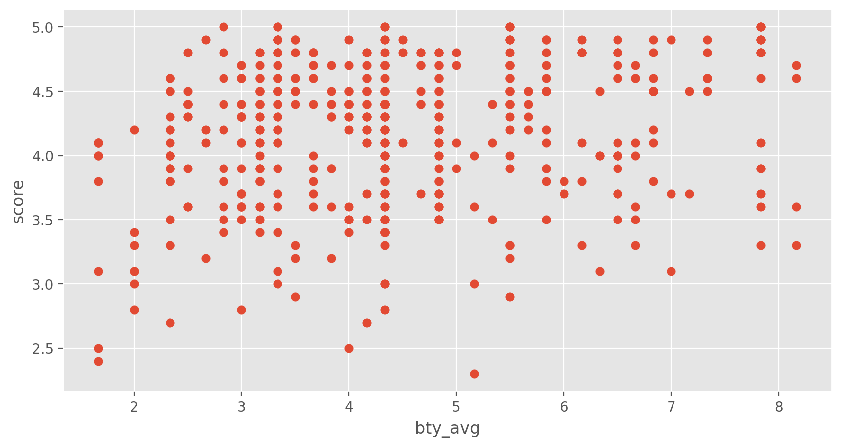
Before we draw conclusions about the trend, compare the number of observations in the data frame with the approximate number of points on the scatterplot. Is anything awry?
Exercise 4
Replot the scatterplot, but this time add jitter on the y- or the x-coordinate. What was misleading about the initial scatterplot?Exercise 5
Let's see if the apparent trend in the plot is something more than natural variation. Fit a linear model calledm_bty to predict average professor score by average beauty rating and add the line to your plot. Write out the equation for the linear model and interpret the slope. Is average beauty score a statistically significant predictor? Does it appear to be a practically significant predictor?
Exercise 6
Use residual plots to evaluate whether the conditions of least squares regression are reasonable. Provide plots and comments for each one (see the Simple Regression Lab for a reminder of how to make these).Multiple linear regression#
The data set contains several variables on the beauty score of the professor: individual ratings from each of the six students who were asked to score the physical appearance of the professors and the average of these six scores. Let’s take a look at the relationship between one of these scores and the average beauty score.
plt.scatter(evals.bty_f1lower, evals.bty_avg)
plt.xlabel('bty_f1lower')
plt.ylabel('bty_avg')
plt.show();
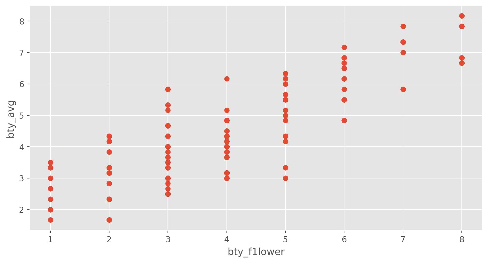
evals.bty_avg.corr(evals.bty_f1lower)
0.843911169214788
As expected the relationship is quite strong - after all, the average score is calculated using the individual scores. We can actually take a look at the relationships between all beauty variables (columns 13 through 19) by plotting pairwise relationships using pairplot() function by seaborn:
import seaborn as sns

sns.pairplot(evals.iloc[:,12:19])
plt.show();
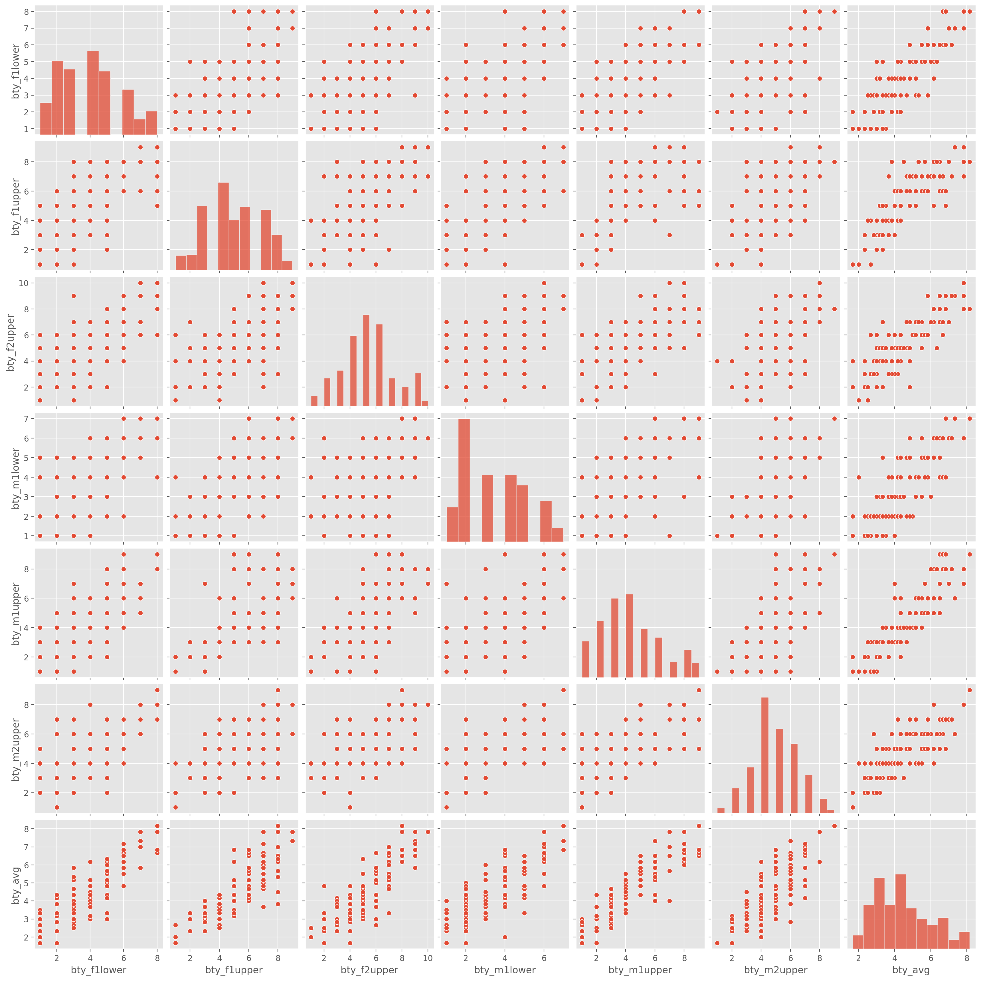
These variables are collinear (correlated), and adding more than one of these variables to the model would not add much value to the model. In this application and with these highly-correlated predictors, it is reasonable to use the average beauty score as the single representative of these variables.
In order to see if beauty is still a significant predictor of professor score after we’ve accounted for the gender of the professor, we can add the gender term into the model.
Since gender is a nominal category feature, we first need to convert gender from having the values of female and male to being an indicator variable called gender_integer that takes a value of 0 for females and a value of 1 for males (Such variables are often referred to as “dummy” variables.). We can use the replace() function for integer-encoding. Before using the replace() function, we need define a mapping between the levels and the integers using a dictionary as below.
level_mapping = {'female': 0, 'male': 1}
Once we define a mapping, we can define a new variable called gender_integer and then perform the integer-encoding using the replace() function.
gender_integer = evals['gender'].copy()
gender_integer = gender_integer.replace(level_mapping)
gender_integer.head(5)
evals['gender_integer'] = gender_integer
import numpy as np
from sklearn.linear_model import LinearRegression
from sklearn.metrics import r2_score

x = evals[['bty_avg','gender_integer']].copy()
y = np.array(evals.score).reshape((-1, 1))

# model initialization
mlinear_model = LinearRegression()
# fit the data
mlinear_model.fit(x, y)
# predict
y_pred = mlinear_model.predict(x)
print('Slope:', mlinear_model.coef_)
print('Intercept:', mlinear_model.intercept_)
print('R-squared:', r2_score(y, y_pred))
Slope: [[0.07415537 0.17238955]]
Intercept: [3.74733824]
R-squared: 0.05912279033681789
Exercise 7
P-values and parameter estimates should only be trusted if the conditions for the regression are reasonable. Verify that the conditions for this model are reasonable using diagnostic plots.Exercise 8
Isbty_avg still a significant predictor of score? Has the addition of gender to the model changed the parameter estimate for bty_avg?
As a result, for females, the parameter estimate is multiplied by zero, leaving the intercept and slope form familiar from simple regression.
\({\hat{score}}\) = \({\hat{\beta}}\)0 + \({\hat{\beta}}\)1 \({*}\) bty_avg + \({\hat{\beta}}\)2 \({*}\) (0) = \({\hat{\beta}}\)0 + \({\hat{\beta}}\)1 \({*}\) bty_avg#
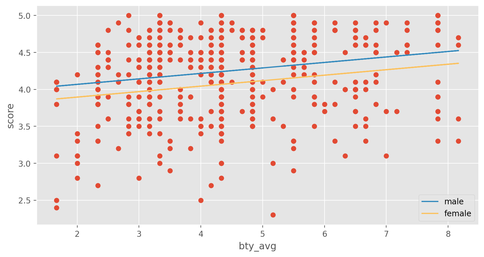
We can plot two lines corresponding to males and females.
plt.scatter(evals.bty_avg, evals.score, label = '')
plt.xlabel('bty_avg')
plt.ylabel('score')

# male
y_male = 3.74733824 + 0.07415537*evals.bty_avg + 0.17238955*1
plt.plot(evals.bty_avg, y_male, color = 'C8', label = 'male')

# female
y_female = 3.74733824 + 0.07415537*evals.bty_avg + 0.17238955*0
plt.plot(evals.bty_avg, y_female, color = 'C4', label = 'female')

plt.legend(loc = 'lower right')
plt.show();
Exercise 9
What is the equation of the line corresponding to males? (Hint: For males, the parameter estimate is multiplied by 1.) For two professors who received the same beauty rating, which gender tends to have the higher course evaluation score?Exercise 10
Create a new model calledm_bty_rank with gender removed and rank added in. Note that the rank variable has three levels: teaching , tenure track , tenured .
The interpretation of the coefficients in multiple regression is slightly different from that of simple regression. The estimate for bty_avg reflects how much higher a group of professors is expected to score if they have a beauty rating that is one point higher while holding all other variables constant. In this case, that translates into considering only professors of the same rank with bty_avg scores that are one point apart.
The search for the best model#
We will start with a full model that predicts professor score based on rank, ethnicity, gender, language of the university where they got their degree, age, proportion of students that filled out evaluations, class size, course level, number of professors, number of credits, average beauty rating, outfit, and picture color.
Exercise 11
Which variable would you expect to have the highest p-value in this model? Why? Hint: Think about which variable would you expect to not have any association with the professor score.Let’s run the model via statsmodels…
import statsmodels.api as sm

m_full = sm.formula.ols(formula = 'score ~ rank + ethnicity + gender + language + age + cls_perc_eval + cls_students + cls_level + cls_profs + cls_credits + bty_avg + pic_outfit + pic_color', data = evals)
multi_reg = m_full.fit()
print(multi_reg.summary())
                            OLS Regression Results
==============================================================================
Dep. Variable:                  score   R-squared:                       0.187
Model:                            OLS   Adj. R-squared:                  0.162
Method:                 Least Squares   F-statistic:                     7.366
Date:                Tue, 23 Jul 2024   Prob (F-statistic):           6.55e-14
Time:                        00:32:54   Log-Likelihood:                -326.52
No. Observations:                 463   AIC:                             683.0
Df Residuals:                     448   BIC:                             745.1
Df Model:                          14
Covariance Type:            nonrobust
=============================================================================================
                                coef    std err          t      P>|t|      [0.025      0.975]
---------------------------------------------------------------------------------------------
Intercept                     4.0952      0.291     14.096      0.000       3.524       4.666
rank[T.tenure track]         -0.1476      0.082     -1.798      0.073      -0.309       0.014
rank[T.tenured]              -0.0973      0.066     -1.467      0.143      -0.228       0.033
ethnicity[T.not minority]     0.1235      0.079      1.571      0.117      -0.031       0.278
gender[T.male]                0.2109      0.052      4.071      0.000       0.109       0.313
language[T.non-english]      -0.2298      0.111     -2.063      0.040      -0.449      -0.011
cls_level[T.upper]            0.0605      0.058      1.051      0.294      -0.053       0.174
cls_profs[T.single]          -0.0147      0.052     -0.282      0.778      -0.117       0.088
cls_credits[T.one credit]     0.5020      0.116      4.330      0.000       0.274       0.730
pic_outfit[T.not formal]     -0.1127      0.074     -1.525      0.128      -0.258       0.033
pic_color[T.color]           -0.2173      0.072     -3.039      0.003      -0.358      -0.077
age                          -0.0090      0.003     -2.872      0.004      -0.015      -0.003
cls_perc_eval                 0.0053      0.002      3.461      0.001       0.002       0.008
cls_students                  0.0005      0.000      1.205      0.229      -0.000       0.001
bty_avg                       0.0400      0.018      2.287      0.023       0.006       0.074
==============================================================================
Omnibus:                       30.719   Durbin-Watson:                   1.410
Prob(Omnibus):                  0.000   Jarque-Bera (JB):               35.095
Skew:                          -0.666   Prob(JB):                     2.40e-08
Kurtosis:                       3.218   Cond. No.                     1.47e+03
==============================================================================

Notes:
[1] Standard Errors assume that the covariance matrix of the errors is correctly specified.
[2] The condition number is large, 1.47e+03. This might indicate that there are
strong multicollinearity or other numerical problems.