SK Part 2: Feature Selection and Ranking

SK Part 2: Feature Selection and Ranking#

The topic of this tutorial is feature selection and ranking (as in “what are the most important 5 features?”). Feature selection is usually an overlooked issue in machine learning. In many cases, using all the descriptive features that are available can lead to excessive computational times, overfitting, and poor performance in general. It’s always a good idea to check to see if we can achieve better performance by employing some sort of feature selection before fitting a model. Feature selection can also be performed in conjunction with the modeling process (as part of a machine learning pipeline), which is discussed in SK Part 5.

Learning Objectives#

Perform feature selection and ranking using the following methods:
- F-score (a statistical filter method)
- Mutual information (an entropy-based filter method)
- Random forest importance (an ensemble-based filter method)
- spFSR (feature selection using stochastic optimisation)
Compare performance of feature selection methods using paired t-tests.

First, let’s discuss some terminology.

The classifier used to assess performance of the feature selection methods is called the “wrapper”. Here, we use the decision tree classifier as the wrapper. As for the sample data, we use the breast cancer Wisconsin dataset.

The first three methods are “filter methods”: they examine the relationship between the descriptive features and the target feature and they select features only once regardless of which classifier shall be used subsequently.

The last method is a “wrapper method”: it selects a different set of features for each wrapper. Wrapper feature selection methods are relatively slow and they need to be executed again when a different wrapper is used. For instance, the best 5 features selected by a wrapper method for a decision tree classifier will probably be different than the best 5 features for the 1-nearest neighbor classifier. However, wrapper methods attempt to solve the “real problem”: “what is the best subset of features when, say, the decision tree classifier is used?”. They usually perform better than the filter methods at the cost of more computational resources and a different set of features for each classifier.

Table of Contents#

Data Preparation
Performance with Full Set of Features
Feature Selection Using F-Score
Feature Selection Using Mutual Information
Feature Selection Using Random Forest Importance
Feature Selection Using spFSR
Performance Comparison Using Paired T-Tests

Data Preparation#

import warnings
warnings.filterwarnings("ignore")

import numpy as np
import pandas as pd
from sklearn.model_selection import cross_val_score, RepeatedStratifiedKFold
import sklearn.metrics as metrics
from sklearn.ensemble import RandomForestClassifier
from sklearn import preprocessing
from sklearn import feature_selection as fs
from sklearn.tree import DecisionTreeClassifier

Let’s load the dataset from the Cloud.

import warnings
warnings.filterwarnings("ignore")

import numpy as np
import pandas as pd
import io
import requests

# so that we can see all the columns
pd.set_option('display.max_columns', None) 

# how to read a csv file from a github account
url_name = 'https://raw.githubusercontent.com/akmand/datasets/master/breast_cancer_wisconsin.csv'
url_content = requests.get(url_name, verify=False).content
df = pd.read_csv(io.StringIO(url_content.decode('utf-8')))

Let’s have a look at the first 5 rows to see what the dataset looks like. Here, the last column “diagnosis” is the target variable.

df.head()

	mean_radius	mean_texture	mean_perimeter	mean_area	mean_smoothness	mean_compactness	mean_concavity	mean_concave_points	mean_symmetry	mean_fractal_dimension	radius_error	texture_error	perimeter_error	area_error	smoothness_error	compactness_error	concavity_error	concave_points_error	symmetry_error	fractal_dimension_error	worst_radius	worst_texture	worst_perimeter	worst_area	worst_smoothness	worst_compactness	worst_concavity	worst_concave_points	worst_symmetry	worst_fractal_dimension	diagnosis
0	17.99	10.38	122.80	1001.0	0.11840	0.27760	0.3001	0.14710	0.2419	0.07871	1.0950	0.9053	8.589	153.40	0.006399	0.04904	0.05373	0.01587	0.03003	0.006193	25.38	17.33	184.60	2019.0	0.1622	0.6656	0.7119	0.2654	0.4601	0.11890	M
1	20.57	17.77	132.90	1326.0	0.08474	0.07864	0.0869	0.07017	0.1812	0.05667	0.5435	0.7339	3.398	74.08	0.005225	0.01308	0.01860	0.01340	0.01389	0.003532	24.99	23.41	158.80	1956.0	0.1238	0.1866	0.2416	0.1860	0.2750	0.08902	M
2	19.69	21.25	130.00	1203.0	0.10960	0.15990	0.1974	0.12790	0.2069	0.05999	0.7456	0.7869	4.585	94.03	0.006150	0.04006	0.03832	0.02058	0.02250	0.004571	23.57	25.53	152.50	1709.0	0.1444	0.4245	0.4504	0.2430	0.3613	0.08758	M
3	11.42	20.38	77.58	386.1	0.14250	0.28390	0.2414	0.10520	0.2597	0.09744	0.4956	1.1560	3.445	27.23	0.009110	0.07458	0.05661	0.01867	0.05963	0.009208	14.91	26.50	98.87	567.7	0.2098	0.8663	0.6869	0.2575	0.6638	0.17300	M
4	20.29	14.34	135.10	1297.0	0.10030	0.13280	0.1980	0.10430	0.1809	0.05883	0.7572	0.7813	5.438	94.44	0.011490	0.02461	0.05688	0.01885	0.01756	0.005115	22.54	16.67	152.20	1575.0	0.1374	0.2050	0.4000	0.1625	0.2364	0.07678	M

Let’s do some pre-processing:

Split the dataset columns into Data and target.
Make target numeric by label-encoding.
Normalize each descriptive feature in Data to be between 0 and 1.

Data = df.drop(columns = 'diagnosis').values
target = df['diagnosis']
Data = preprocessing.MinMaxScaler().fit_transform(Data)
target = preprocessing.LabelEncoder().fit_transform(target)

Performance with Full Set of Features#

As wrapper, we use the decision tree classifier with default values.

clf = DecisionTreeClassifier(random_state=999)

First, we would like to assess performance using all the features in the dataset. For assessment, we shall use stratified 5-fold cross-validation with 3 repetitions. We set the random state to 999 so that our results can be replicated and verified later on exactly as they are.

cv_method = RepeatedStratifiedKFold(n_splits=5, 
                                     n_repeats=3,
                                     random_state=999)

For scoring, we use the accuracy score.

scoring_metric = 'accuracy'

Let’s perform the cross-validation using the cross_val_score function.

cv_results_full = cross_val_score(estimator=clf,
                             X=Data,
                             y=target, 
                             cv=cv_method, 
                             scoring=scoring_metric)

The array cv_results_full contains 15 values corresponding to each one of the 3-repetition/ 5-fold combinations.

cv_results_full

array([0.92105263, 0.95614035, 0.9122807 , 0.92105263, 0.97345133,
       0.94736842, 0.92982456, 0.87719298, 0.92105263, 0.92920354,
       0.9122807 , 0.92982456, 0.92105263, 0.95614035, 0.9380531 ])

We compute the average cross-validation performance as the mean of the cv_results_full array.

cv_results_full.mean().round(3)

np.float64(0.93)

Let’s now select the best 5 features in the dataset using different methods.

num_features = 5

Feature Selection Using F-Score#

The F-Score method is a filter feature selection method that looks at the relationship between each descriptive feature and the target feature using the F-distribution.

The code below returns the indices of the 5 features that have the highest F-Score value sorted from the highest to the lowest. Pay attention that the wrapper is not used in any way when selecting features using the F-Score method.

In some cases, the F-Score will be “NaN” for some features due to technical reasons (related to the nature of the F-distribution). For this reason, we will convert any “NaN” value to zero for a correct result via the np.nan_to_num() method.

fs_fit_fscore = fs.SelectKBest(fs.f_classif, k=num_features)
fs_fit_fscore.fit_transform(Data, target)
fs_indices_fscore = np.argsort(np.nan_to_num(fs_fit_fscore.scores_))[::-1][0:num_features]
fs_indices_fscore

array([27, 22,  7, 20,  2])

Let’s see what these 5 best features are.

best_features_fscore = df.columns[fs_indices_fscore].values
best_features_fscore

array(['worst_concave_points', 'worst_perimeter', 'mean_concave_points',
       'worst_radius', 'mean_perimeter'], dtype=object)

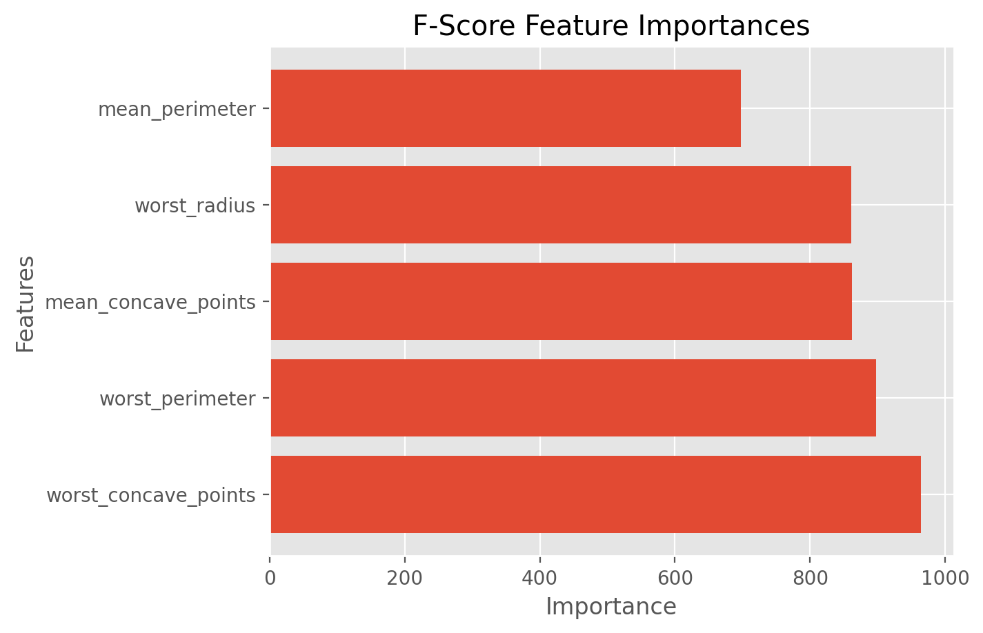
Based on the F-Scores, we observe that, out of the top 5 features, the most important feature is “worst_concave_points” and the least important feature is “mean_perimeter”.

The F-Score importances of these features are given below.

feature_importances_fscore = fs_fit_fscore.scores_[fs_indices_fscore]
feature_importances_fscore

array([964.38539345, 897.94421886, 861.67602001, 860.78170699,
       697.23527248])

We define a function for plotting so that we can plot other importance types as well corresponding to different feature selection methods.

import matplotlib.pyplot as plt
%matplotlib inline 
%config InlineBackend.figure_format = 'retina'
plt.style.use("ggplot")

def plot_imp(best_features, scores, method_name):   
    plt.barh(best_features, scores)
    plt.title(method_name + ' Feature Importances')
    plt.xlabel("Importance")
    plt.ylabel("Features")
    plt.show()
    

plot_imp(best_features_fscore, feature_importances_fscore, 'F-Score')

../_images/0eb9d8ca3044962acc2daa7488d86d6a8bf89b45e1c5ac050328a4ac14735add.png

We can select those features from the set of descriptive features Data using slicing as shown below.

Data[:, fs_indices_fscore].shape

(569, 5)

Let’s now assess performance of this feature selection method using cross validation with the decision tree classifier.

cv_results_fscore = cross_val_score(estimator=clf,
                             X=Data[:, fs_indices_fscore],
                             y=target, 
                             cv=cv_method, 
                             scoring=scoring_metric)
cv_results_fscore.mean().round(3)

np.float64(0.926)

Feature Selection Using Mutual Information#

The mutual information method is a filter feature selection method that looks at the relationship between each descriptive feature and the target feature using the concept of entropy.

The code below returns the indices of the 5 features that have the highest mutual information value. As in the F-score method, the wrapper is not used in any way when selecting features using the mutual information method.

fs_fit_mutual_info = fs.SelectKBest(fs.mutual_info_classif, k=num_features)
fs_fit_mutual_info.fit_transform(Data, target)
fs_indices_mutual_info = np.argsort(fs_fit_mutual_info.scores_)[::-1][0:num_features]
best_features_mutual_info = df.columns[fs_indices_mutual_info].values
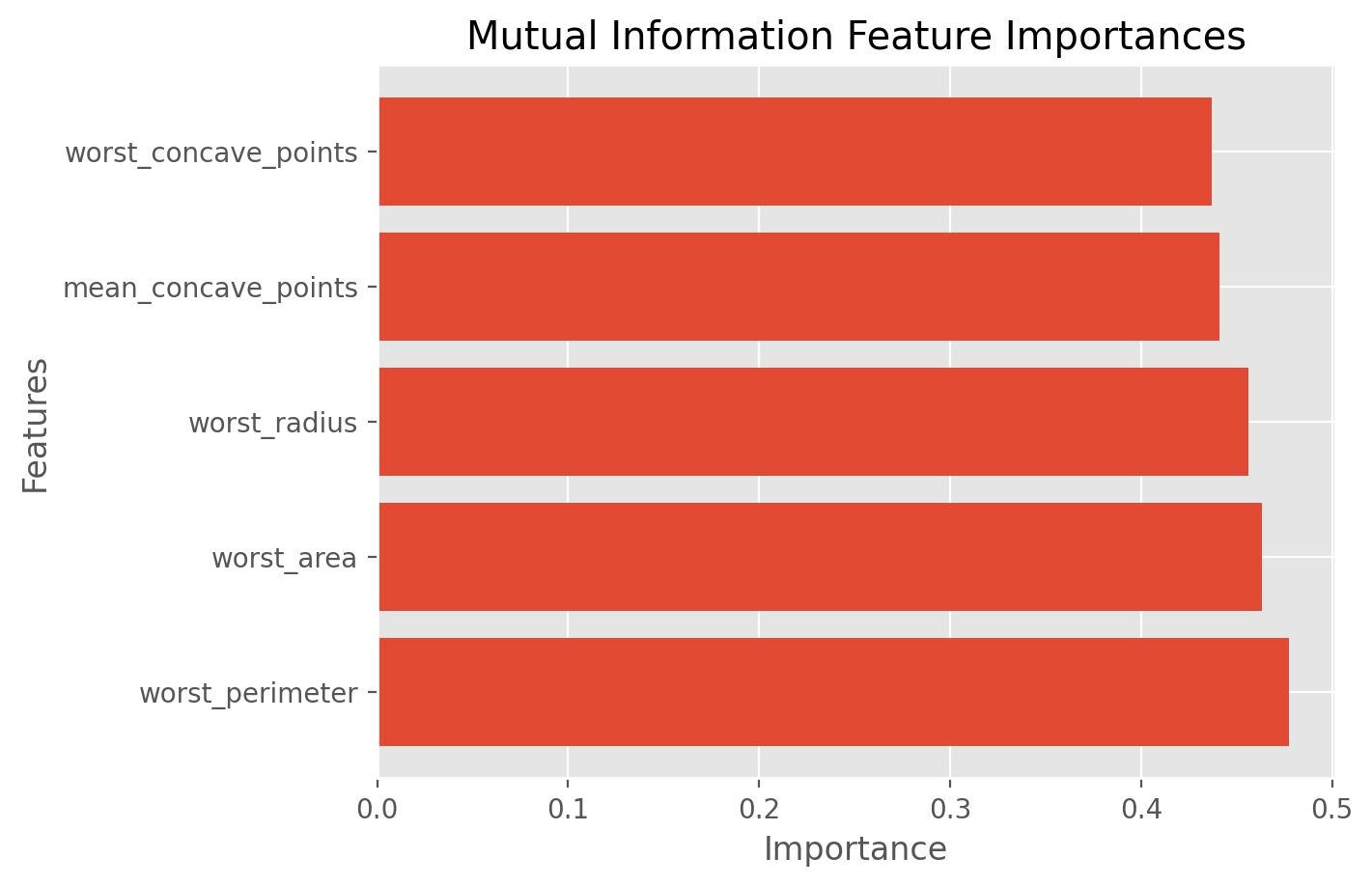
best_features_mutual_info

array(['worst_perimeter', 'worst_area', 'worst_radius',
       'mean_concave_points', 'worst_concave_points'], dtype=object)

feature_importances_mutual_info = fs_fit_mutual_info.scores_[fs_indices_mutual_info]
feature_importances_mutual_info

array([0.47764827, 0.4632881 , 0.45627324, 0.44107263, 0.4368373 ])

plot_imp(best_features_mutual_info, feature_importances_mutual_info, 'Mutual Information')

../_images/d1d98b8c297f0419f37dc7d44d2f062f3b05ac4939e4cfc24aa4fcc1837ae6e1.png

Now let’s evaluate the performance of these features.

cv_results_mutual_info = cross_val_score(estimator=clf,
                             X=Data[:, fs_indices_mutual_info],
                             y=target, 
                             cv=cv_method, 
                             scoring=scoring_metric)
cv_results_mutual_info.mean().round(3)

np.float64(0.919)

Feature Selection Using Random Forest Importance#

The random forest importance (RFI) method is a filter feature selection method that uses the total decrease in node impurities from splitting on a particular feature as averaged over all decision trees in the ensemble. For classification, the node impurity is measured by the Gini index and for regression, it is measured by residual sum of squares.

Let’s perform RFI feature selection using 100 trees.

model_rfi = RandomForestClassifier(n_estimators=100)
model_rfi.fit(Data, target)
fs_indices_rfi = np.argsort(model_rfi.feature_importances_)[::-1][0:num_features]

Here are the best features selected by RFI.

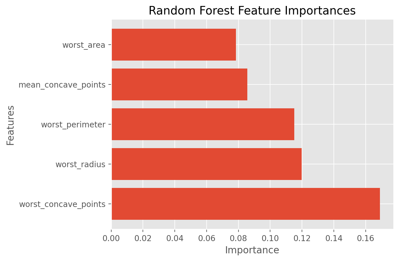
best_features_rfi = df.columns[fs_indices_rfi].values
best_features_rfi

array(['worst_concave_points', 'worst_radius', 'worst_perimeter',
       'mean_concave_points', 'worst_area'], dtype=object)

feature_importances_rfi = model_rfi.feature_importances_[fs_indices_rfi]
feature_importances_rfi

array([0.16911595, 0.11984545, 0.11509717, 0.08568064, 0.07844842])

plot_imp(best_features_rfi, feature_importances_rfi, 'Random Forest')

../_images/a00f8f02fbadfe48d6c035bff05fb7d60c981be7fb3578f811501b915ff9f82e.png

Now let’s evaluate the performance of these features.

cv_results_rfi = cross_val_score(estimator=clf,
                             X=Data[:, fs_indices_rfi],
                             y=target, 
                             cv=cv_method, 
                             scoring=scoring_metric)
cv_results_rfi.mean().round(3)

np.float64(0.925)

Feature Selection Using spFSR#

spFSR is a new wrapper-based feature selection method that uses binary stochastic approximation. Please refer to this journal article paper for more information on this method.

First, you need to make sure that you download and copy the Python file spFSR.py under the same directory as your Jupyter notebook so that the import works correctly. You can download this file from this link.

Let’s define an SpFSR object with our feature selection problem with ‘accuracy’ as our performance metric. Let’s run spFSR in the wrapper mode by setting wrapper=clf.

Please keep in mind that spFSR can be used as a filter-based feature selection method as well so that the selected features do not depend on the intended classifier. For this to work, just set the wrapper parameter to None. For more details, please see this example.

# pay attention to capitalization below!
from spFSR import SpFSR

# set the engine parameters
# pred_type needs to be 'c' for classification and 'r' for regression datasets
sp_engine = SpFSR(x=Data, y=target, pred_type='c', wrapper=clf, scoring='accuracy')

Let’s now run the spFSR method and the indices of the best features.

np.random.seed(999)
sp_output = sp_engine.run(num_features=num_features).results

SpFSR-INFO: Wrapper: DecisionTreeClassifier(random_state=999)
SpFSR-INFO: Hot start: True
SpFSR-INFO: Hot start range: 0.2
SpFSR-INFO: Feature weighting: False
SpFSR-INFO: Scoring metric: accuracy
SpFSR-INFO: Number of jobs: 1
SpFSR-INFO: Number of observations in the dataset: 569
SpFSR-INFO: Number of observations used: 569
SpFSR-INFO: Number of features available: 30
SpFSR-INFO: Number of features to select: 5
SpFSR-INFO: iter_no: 0, num_ft: 5, value: 0.924, st_dev: 0.026, best: 0.924 @ iter_no 0
SpFSR-INFO: ===> iter_no: 4, same feature stall limit reached, initializing search...
SpFSR-INFO: iter_no: 10, num_ft: 5, value: 0.93, st_dev: 0.016, best: 0.948 @ iter_no 6
SpFSR-INFO: iter_no: 20, num_ft: 5, value: 0.939, st_dev: 0.016, best: 0.948 @ iter_no 6
SpFSR-INFO: ===> iter_no: 23, same feature stall limit reached, initializing search...
SpFSR-INFO: iter_no: 30, num_ft: 5, value: 0.928, st_dev: 0.032, best: 0.948 @ iter_no 6
SpFSR-INFO: iter_no: 40, num_ft: 5, value: 0.933, st_dev: 0.02, best: 0.948 @ iter_no 6
SpFSR-INFO: ===> iter_no: 41, same feature stall limit reached, initializing search...
SpFSR-INFO: iter_no: 50, num_ft: 5, value: 0.927, st_dev: 0.022, best: 0.948 @ iter_no 6
SpFSR-INFO: iter_no: 60, num_ft: 5, value: 0.929, st_dev: 0.026, best: 0.948 @ iter_no 6
SpFSR-INFO: iter_no: 70, num_ft: 5, value: 0.919, st_dev: 0.021, best: 0.948 @ iter_no 6
SpFSR-INFO: ===> iter_no: 72, same feature stall limit reached, initializing search...
SpFSR-INFO: iter_no: 80, num_ft: 5, value: 0.943, st_dev: 0.023, best: 0.948 @ iter_no 6
SpFSR-INFO: ===> iter_no: 85, same feature stall limit reached, initializing search...
SpFSR-INFO: iter_no: 90, num_ft: 5, value: 0.923, st_dev: 0.02, best: 0.948 @ iter_no 6
SpFSR-INFO: iter_no: 100, num_ft: 5, value: 0.931, st_dev: 0.026, best: 0.948 @ iter_no 6
SpFSR-INFO: SpFSR completed in 0.12 minutes.
SpFSR-INFO: Best value = 0.948 with 5 features and 100 total iterations.

Let’s get the indices of the best features.

fs_indices_spfsr = sp_output.get('selected_features')
fs_indices_spfsr

[23, 27, 26, 21, 2]

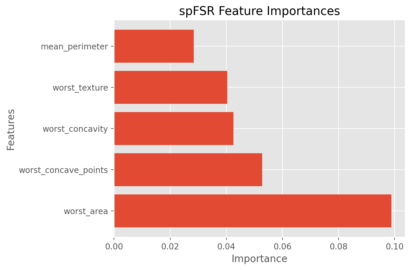
Let’s have a look at the top 5 features selected by spFSR.

best_features_spfsr = df.columns[fs_indices_spfsr]
best_features_spfsr

Index(['worst_area', 'worst_concave_points', 'worst_concavity',
       'worst_texture', 'mean_perimeter'],
      dtype='object')

feature_importances_spfsr = sp_output.get('selected_ft_importance')
feature_importances_spfsr

array([0.09887883, 0.05283565, 0.04254586, 0.0403938 , 0.02842053])

plot_imp(best_features_spfsr, feature_importances_spfsr, 'spFSR')

../_images/9893a14d54822b5c7195d41c8d5fdb7db627430085f72a26f27c646399db50c9.png

Finally, let’s evaluate the performance of the spFSR feature selection method.

cv_results_spfsr = cross_val_score(estimator=clf,
                             X=Data[:, fs_indices_spfsr],
                             y=target, 
                             cv=cv_method, 
                             scoring=scoring_metric)
cv_results_spfsr.mean().round(3)

np.float64(0.941)

We observe that we get a cross-validation accuracy of 94.4% with spFSR with just 5 features. Recall that the cross-validation accuracy with the full set of features is 93%. So, in this particular case, it is remarkable that we can achieve even slightly better results with 5 features selected by spFSR as opposed to using all the 30 features. However, we will need to conduct a t-test to determine if this difference is statistically significant or not.

Performance Comparison Using Paired T-Tests#

For performance assessment, we used repeated cross-validation. However, cross-validation is a random process and we need statistical tests in order to determine if any difference between the performance of any two feature selection methods is statistically significant; or if it is within the sample variation and the difference is statistically insignificant.

Since we fixed the random state to be same for all cross-validation procedures, all feature selection methods were fitted and then tested on exactly the same data partitions. This indicates that our experiments were actually paired. Conducting experiments in a paired fashion reduces the variability significantly compared to conducting experiments in an independent fashion.

Let’s now conduct paired t-tests to see which differences between full set of features, filter methods, and spFSR are statistically significant. Let’s first remind ourselves the performances.

print('Full Set of Features:', cv_results_full.mean().round(3))
print('F-Score:', cv_results_fscore.mean().round(3))
print('Mutual Information:', cv_results_mutual_info.mean().round(3))
print('RFI:', cv_results_rfi.mean().round(3))
print('spFSR:', cv_results_spfsr.mean().round(3)) 

Full Set of Features: 0.93
F-Score: 0.926
Mutual Information: 0.919
RFI: 0.925
spFSR: 0.941

The above results indicate that spFSR outperforms the other FS methods. However, we need to perform some statistical tests to check to see if this difference is indeed statistically significant.

For a paired t-test in Python, we use the stats.ttest_rel function inside the scipy module and look at the p-values. At a 95% significance level, if the p-value is smaller than 0.05, we can conclude that the difference is statistically significant.

from scipy import stats
print(stats.ttest_rel(cv_results_spfsr, cv_results_fscore).pvalue.round(3))
print(stats.ttest_rel(cv_results_spfsr, cv_results_mutual_info).pvalue.round(3))
print(stats.ttest_rel(cv_results_spfsr, cv_results_rfi).pvalue.round(3))

019
014
054

Since all p-values are below 0.05, we conclude that spFSR is statistically better than the other FS methods. Next, let’s see if spFSR performance is better than that with full set of features.

stats.ttest_rel(cv_results_spfsr, cv_results_full).pvalue.round(3)

np.float64(0.103)

For spFSR vs. full set of features, we observe a p-value above 0.05, indicating that the difference is not statically significant. Thus, spFSR with 5 features performs statistically the same as the full set of features, at least for the decision tree classifier.

Note: In this notebook, we use all the data to train the feature selection methods and then tested them again on the entire dataset using cross-validation due to the smallness of the dataset to work with. Despite its simplicity, this approach potentially results in overfitting. In order to mitigate this issue, a more appropriate approach would be to perform this comparison within a train/ test split approach. Specifically, we can split the entire data into two partitions, a train and a test data. We can find the top features using the train data using cross-validation. Next, we can assess the performance of these features on the test data, again using cross-validation.