Pandas

Pandas#

The Pandas module is Python’s fundamental data analytics library and it provides high-performance, easy-to-use data structures and tools for data analysis. Pandas allows for creating pivot tables, computing new columns based on other columns, etc. Pandas also facilitates grouping rows by column values and joining tables as in SQL.

A good cheat sheet for Pandas can be found here.

Pandas is a very comprehensive and mature module that can be used for advanced data analytics, and this tutorial presents just a very basic overview of Pandas’ capabilities.

Before we start, let’s suppress warnings as they can get annoying sometimes.

import warnings
warnings.filterwarnings('ignore')

Let’s import Pandas with the usual convention as pd and NumPy as np.

import pandas as pd
import numpy as np

Series and Data Frames#

There are two main data structures in Pandas: Series and DataFrame.

Series is like a Python list: it is a one-dimensional data structure that can store values with labels (or index). We can initialize a Series with a list as below.

x = pd.Series([34, 23, -5, 0])
print(x)

  34
  23
  -5
   0
dtype: int64

If you would like to see the list of methods that you can use with a Series, use the code completion feature in Jupyter Notebook: type “x.” in a cell and then hit the Tab button.

A DataFrame is just a table with rows and columns, much like an Excel spreadsheet.

An easy way to create a DataFrame object is by using a dictionary:

data = {'name': ['Mary', 'David', 'Jack', 'John', 'Robin'],
        'state': ['VIC', 'NSW', 'VIC', 'SA', 'QLD'],
        'birthyear': [1980, 1992, 2000, 1980, 1995]}
df = pd.DataFrame(data)
df

	name	state	birthyear
0	Mary	VIC	1980
1	David	NSW	1992
2	Jack	VIC	2000
3	John	SA	1980
4	Robin	QLD	1995

An alternative is to first define an empty data frame with column names and then append rows to it as dictionaries whose keys are the columns.

df = pd.DataFrame(columns=['name', 'state', 'birthyear'])

# Add rows using loc with dictionaries
df.loc[len(df)] = {'name': 'Mary', 'state': 'VIC', 'birthyear': 1980}
df.loc[len(df)] = {'name': 'David', 'state': 'NSW', 'birthyear': 1992}

df

	name	state	birthyear
0	Mary	VIC	1980
1	David	NSW	1992

A second alternative, which is a bit shorter, is to append rows as lists at the end of the data frame.

df = pd.DataFrame(columns=['name', 'state', 'birthyear'])
df.loc[len(df)] = ['Mary', 'VIC', 1980]
df.loc[len(df)] = ['David', 'NSW', 1992]

df

	name	state	birthyear
0	Mary	VIC	1980
1	David	NSW	1992

This tutorial will mostly focus on data frames, since real-world datasets are generally multi-dimensional tables rather than just one dimensional arrays.

Loading Data: Course Grades#

This sample data contains course assessment results and students’ final grades (Pass or Fail) for a class with 40 students.

Student ID: Unique ID number for each student in the data.
Gender: The gender of student.
Project Phase 1: The mark student received by completing the first part of project. The marks are out of 20.
Project Phase 2: The mark student received by completing the second part of project. The marks are out of 30.
Mid-Semester Test: The mark student received from the mid-semester test. The marks are out of 100.
Final Exam: The mark student received from the final exam. The marks are out of 100.
Grade: The grade student received indicating whether they passed or failed.

Now let’s load the data into a DataFrame object from the Cloud.

import warnings
warnings.filterwarnings("ignore")

import io
import requests

# so that we can see all the columns
pd.set_option('display.max_columns', None) 

# how to read a csv file from a github account
url_name = 'https://raw.githubusercontent.com/akmand/datasets/master/sample_grades.csv'
url_content = requests.get(url_name, verify=False).content
grades = pd.read_csv(io.StringIO(url_content.decode('utf-8')))

# alternatively, you can download this CSV file to 
# where this notebook is on your computer
# and then use the read_csv() method:
# ### grades = pd.read_csv('sample_grades.csv', header=0)

Data Exploration#

Preview#

There are different approaches to viewing the data we are interested in exploring.

The method head() prints the first five rows by default.

grades.head()

	Student ID	Gender	Project Phase 1	Project Phase 2	Mid-Semester Test	Final Exam	Grade
0	101	Male	18.25	15.5	94	61.0	PA
1	102	Female	17.75	30.0	79	62.0	PA
2	103	Male	0.00	0.0	78	15.0	NN
3	104	Male	20.00	25.0	69	65.0	PA
4	105	Male	18.75	30.0	96	51.0	PA

Alternatively, we can define the number of header rows we want to print.

grades.head(2)

	Student ID	Gender	Project Phase 1	Project Phase 2	Mid-Semester Test	Final Exam	Grade
0	101	Male	18.25	15.5	94	61.0	PA
1	102	Female	17.75	30.0	79	62.0	PA

tail() prints the last five rows by default.

grades.tail()

	Student ID	Gender	Project Phase 1	Project Phase 2	Mid-Semester Test	Final Exam	Grade
35	136	Male	18.50	22.0	26	68.0	PA
36	137	Female	20.00	26.0	89	63.0	PA
37	138	Male	18.75	30.0	59	52.0	PA
38	139	Male	19.00	30.0	70	NaN	PA
39	140	Male	20.00	29.0	84	77.0	PA

sample() randomly selects rows from the entire data.

grades.sample(5, random_state=99)

	Student ID	Gender	Project Phase 1	Project Phase 2	Mid-Semester Test	Final Exam	Grade
25	126	Female	20.00	22.5	83	56.0	PA
36	137	Female	20.00	26.0	89	63.0	PA
29	130	Male	19.50	13.0	62	39.0	NN
22	123	Male	19.75	30.0	74	61.0	PA
28	129	Male	20.00	30.0	64	86.0	PA

Sorting#

We can sort the data with respect to a particular column by calling sort_values(). Let’s sort the data by Final Exam scores in descending order.

If you want the sorting to be permanent, you must specifically set the inplace argument to True. This is a fundamental rule in Pandas: in most cases, if you don’t set the inplace argument to True, you will need to set the output of the command to another variable to save its effect.

Another nice feature of Pandas is method chaining: notice below how we chain two methods together.

grades.sort_values(by='Final Exam', ascending=False).head()

	Student ID	Gender	Project Phase 1	Project Phase 2	Mid-Semester Test	Final Exam	Grade
27	128	Female	20.0	30.00	84	91.0	PA
28	129	Male	20.0	30.00	64	86.0	PA
26	127	Female	20.0	35.00	84	83.0	PA
14	115	Male	19.5	26.00	100	79.0	PA
13	114	Male	20.0	22.75	85	78.0	PA

Summary#

The function shape counts the number of rows and columns. Thus, number of rows and columns can be obtained as grade.shape[0] and grade.shape[1] respectively.

grades.shape

(40, 7)

info() provides a concise summary of the columns.

grades.info()

<class 'pandas.core.frame.DataFrame'>
RangeIndex: 40 entries, 0 to 39
Data columns (total 7 columns):
 #   Column             Non-Null Count  Dtype  
---  ------             --------------  -----  
 0   Student ID         40 non-null     int64  
 1   Gender             37 non-null     object 
 2   Project Phase 1    40 non-null     float64
 3   Project Phase 2    37 non-null     float64
 4   Mid-Semester Test  40 non-null     int64  
 5   Final Exam         36 non-null     float64
 6   Grade              40 non-null     object 
dtypes: float64(3), int64(2), object(2)
memory usage: 2.3+ KB

describe() generates descriptive statistics. Keep in mind that this function excludes null values.

grades.describe()

	Student ID	Project Phase 1	Project Phase 2	Mid-Semester Test	Final Exam
count	40.000000	40.000000	37.000000	40.000000	36.000000
mean	120.500000	16.987500	23.750000	72.100000	56.055556
std	11.690452	5.964626	7.509716	19.664885	20.520296
min	101.000000	0.000000	0.000000	26.000000	6.000000
25%	110.750000	17.687500	20.000000	59.750000	45.500000
50%	120.500000	19.500000	25.500000	76.000000	60.000000
75%	130.250000	20.000000	30.000000	86.000000	71.750000
max	140.000000	20.000000	35.000000	100.000000	91.000000

To ensure all the columns are listed (including categoricals), we can add the include = all parameter.

grades.describe(include='all')

	Student ID	Gender	Project Phase 1	Project Phase 2	Mid-Semester Test	Final Exam	Grade
count	40.000000	37	40.000000	37.000000	40.000000	36.000000	40
unique	NaN	4	NaN	NaN	NaN	NaN	2
top	NaN	Male	NaN	NaN	NaN	NaN	PA
freq	NaN	22	NaN	NaN	NaN	NaN	29
mean	120.500000	NaN	16.987500	23.750000	72.100000	56.055556	NaN
std	11.690452	NaN	5.964626	7.509716	19.664885	20.520296	NaN
min	101.000000	NaN	0.000000	0.000000	26.000000	6.000000	NaN
25%	110.750000	NaN	17.687500	20.000000	59.750000	45.500000	NaN
50%	120.500000	NaN	19.500000	25.500000	76.000000	60.000000	NaN
75%	130.250000	NaN	20.000000	30.000000	86.000000	71.750000	NaN
max	140.000000	NaN	20.000000	35.000000	100.000000	91.000000	NaN

We can also use the following functions to summarize the data. All these methods exclude null values by default.

count() to count the number of elements.
value_counts() to get a frequency distribution of unique values.
nunique() to get the number of unique values.
mean() to calculate the arithmetic mean of a given set of numbers.
std() to calculate the sample standard deviation of a given set of numbers.
max() to return the maximum of the provided values.
min() to return minimum of the provided values.

grades.count()

Student ID           40
Gender               37
Project Phase 1      40
Project Phase 2      37
Mid-Semester Test    40
Final Exam           36
Grade                40
dtype: int64

grades['Gender'].value_counts()

Gender
Male      22
Female    13
M          1
F          1
Name: count, dtype: int64

grades['Gender'].nunique()

grades['Final Exam'].mean()

np.float64(56.05555555555556)

grades['Mid-Semester Test'].std()

np.float64(19.66488475195551)

grades['Project Phase 2'].max()

np.float64(35.0)

grades['Project Phase 1'].min()

np.float64(0.0)

Selecting specific columns#

When there are many columns, we may prefer to select only the ones we are interested in. Let’s say we want to select the “Gender” and the “Grade” columns only.

# notice the double brackets
grades[['Gender', 'Grade']].head()

	Gender	Grade
0	Male	PA
1	Female	PA
2	Male	NN
3	Male	PA
4	Male	PA

We can also get a single column as a Series object from a data frame.

# notice the single bracket
gender_series = grades['Gender']

type(gender_series)

pandas.core.series.Series

gender_series.head()

    Male
  Female
    Male
    Male
    Male
Name: Gender, dtype: object

Filtering for particular values#

We can subset the data based on a particular criterion. Let’s say we want the list of students who have failed this class.

grades[grades['Grade'] == 'NN']

	Student ID	Gender	Project Phase 1	Project Phase 2	Mid-Semester Test	Final Exam	Grade
2	103	Male	0.00	0.0	78	15.0	NN
8	109	M	18.00	23.0	50	33.0	NN
12	113	Female	0.00	NaN	67	NaN	NN
16	117	NaN	15.75	10.0	81	34.0	NN
17	118	Male	12.50	10.0	30	22.0	NN
18	119	Male	17.50	20.0	61	31.0	NN
21	122	Female	20.00	23.0	37	25.0	NN
29	130	Male	19.50	13.0	62	39.0	NN
30	131	Male	0.00	NaN	60	NaN	NN
31	132	Female	17.50	20.0	42	47.0	NN
34	135	Male	20.00	30.0	61	6.0	NN

We could also filter based on multiple conditions. Let’s see who failed the class even though their final exam scores were higher than 45, but let’s only look at a few of the columns using the loc method.

grades.loc[(grades['Grade'] == 'NN') & (grades['Final Exam'] > 45), ['Student ID', 'Final Exam', 'Grade']]

	Student ID	Final Exam	Grade
31	132	47.0	NN

Now let’s select the last 2 columns and all the rows between 10 and 15 using the iloc method. Notice the use of the negative sign for negative indexing.

grades.iloc[10:16, -2:]

	Final Exam	Grade
10	52.0	PA
11	NaN	PA
12	NaN	NN
13	78.0	PA
14	79.0	PA
15	52.0	PA

Group By#

Pandas allows aggregation of data into groups to run calculations over each group. Let’s group the data by Grade:

grades.groupby(['Grade']).count()

	Student ID	Gender	Project Phase 1	Project Phase 2	Mid-Semester Test	Final Exam
Grade
NN	11	10	11	9	11	9
PA	29	27	29	28	29	27

Here, the size() method makes more sense.

grades.groupby(['Grade']).size()

Grade
NN    11
PA    29
dtype: int64

This time, let’s first group by Gender and then by Grade.

grades.groupby(['Gender','Grade']).count()

		Student ID	Project Phase 1	Project Phase 2	Mid-Semester Test	Final Exam
Gender	Grade
F	PA	1	1	1	1	1
Female	NN	3	3	2	3	2
Female	PA	10	10	9	10	9
M	NN	1	1	1	1	1
Male	NN	6	6	5	6	5
Male	PA	16	16	16	16	15

Notice that there are unexpected multiple levels defining the same category (e.g., F also represents Female). We will take care of this in Data Manipulation section.

So, how do we make the above grouping a data frame? For this, we use the reset_index method.

grades.groupby(['Gender','Grade']).count().reset_index()

	Gender	Grade	Student ID	Project Phase 1	Project Phase 2	Mid-Semester Test	Final Exam
0	F	PA	1	1	1	1	1
1	Female	NN	3	3	2	3	2
2	Female	PA	10	10	9	10	9
3	M	NN	1	1	1	1	1
4	Male	NN	6	6	5	6	5
5	Male	PA	16	16	16	16	15

Data Manipulation#

Handling missing values#

Dealing with missing values is a time consuming but crucial task. We should first identify the missing values and then try to determine why they are missing.

There are two basic strategies to handle missing values:

Remove rows and columns with missing values.
Impute missing values, replacing them with predefined values.

Missing values are a bit complicated in Python as they can be denoted by either “na” or “null” in Pandas (both mean the same thing). Furthermore, NumPy denotes missing values as “NaN” (that is, “not a number”).

First, let’s count the number of missing values in each column.

grades.isna().sum()

Student ID           0
Gender               3
Project Phase 1      0
Project Phase 2      3
Mid-Semester Test    0
Final Exam           4
Grade                0
dtype: int64

The function dropna() drops rows with at least one missing value.

grades_no_na = grades.dropna()
grades_no_na.shape

(33, 7)

grades_no_na.isna().sum()

Student ID           0
Gender               0
Project Phase 1      0
Project Phase 2      0
Mid-Semester Test    0
Final Exam           0
Grade                0
dtype: int64

Now let’s look at the Gender column.

grades['Gender'].value_counts()

Gender
Male      22
Female    13
M          1
F          1
Name: count, dtype: int64

grades['Gender'].isna().sum()

np.int64(3)

So this column has 3 missing values. Let’s use the fillna() method to replace these missing values with “Unknown”:

grades['Gender'].fillna('Unknown', inplace=True)

# this also works:
# ## grades[['Gender']] = grades[['Gender']].fillna('Unknown')

grades['Gender'].value_counts()

Gender
Male       22
Female     13
Unknown     3
M           1
F           1
Name: count, dtype: int64

Let’s go back and check the missing values in our modified data.

grades.isna().sum()

Student ID           0
Gender               0
Project Phase 1      0
Project Phase 2      3
Mid-Semester Test    0
Final Exam           4
Grade                0
dtype: int64

Some assessments have missing values. We know for a fact that these missing values are due to students missing these assessments, and therefore we set these missing values to zero.

grades = grades.fillna(0)

We can now confirm that there are no more missing values.

grades.isna().sum()

Student ID           0
Gender               0
Project Phase 1      0
Project Phase 2      0
Mid-Semester Test    0
Final Exam           0
Grade                0
dtype: int64

Handling irregular cardinality#

The cardinality is the number of different values we have for a particular feature. Sometimes we might have unexpected number of distinct values for a feature and this is called irregular cardinality. Let’s start by counting the unique number of observations for each column by using the nunique() method:

grades.nunique()

Student ID           40
Gender                5
Project Phase 1      15
Project Phase 2      19
Mid-Semester Test    34
Final Exam           31
Grade                 2
dtype: int64

First, it is clear that all the values in the Student ID column are unique for each student. Therefore, we will remove it since ID-type columns are not useful in statistical modeling.

grades.drop(columns=['Student ID'], inplace=True)

Next, we notice Gender has a cardinality of 4, which is more than expected. This issue often arises when multiple levels are used to represent the same thing (e.g., M, male, MALE, Male all represent the “male” gender). For Gender, in this case, there should be only three different values: Female, Male, and Unknown. Let’s print the unique elements in Gender using the value_counts() method:

grades['Gender'].value_counts()

Gender
Male       22
Female     13
Unknown     3
M           1
F           1
Name: count, dtype: int64

Let’s use the replace() method to replace all the problematic levels to a standard set of levels.

grades.replace(['M', 'male'], 'Male', inplace=True)

grades.replace(['F', 'female'], 'Female', inplace=True)

Let’s check again the unique elements in Gender.

grades['Gender'].value_counts()

Gender
Male       23
Female     14
Unknown     3
Name: count, dtype: int64

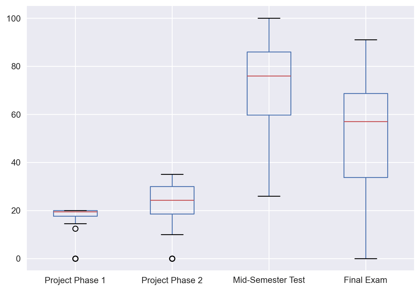
Detecting outliers#

Outliers are values that significantly differ from other values and they lie far away from the central tendency of a variable. The best way to visually detect outliers is by using boxplots. Pandas allows for direct visualization of a data frame’s columns.

First, let’s prepare the plotting environment as Pandas’ plotting functions actually use Matplotlib.

import numpy as np
import matplotlib.pyplot as plt
%matplotlib inline 
%config InlineBackend.figure_format = 'retina'
plt.style.use("seaborn-v0_8")

grades.boxplot(column=['Project Phase 1', 'Project Phase 2', 'Mid-Semester Test', 'Final Exam']);

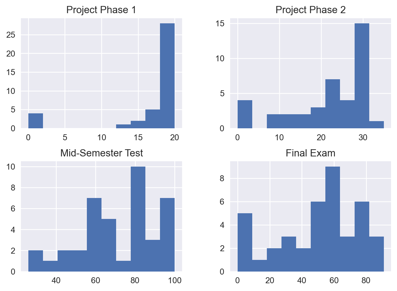
../_images/82b6c21f2e88e013ac0be62547cf657d8df1b618e50df03d11c9afd53c25fa5b.png

Alternatively, we can examine the histogram of these columns.

grades.hist(column=['Project Phase 1', 'Project Phase 2', 'Mid-Semester Test', 'Final Exam']);

../_images/539b8c669bd3a3e35b9f803d063f8f0ea83464821a35522e3dfa51f8a0060aa0.png

Saving a DataFrame#

Pandas allows for saving DataFrame objects in various formats, including CSV, Excel, JSON, HTML, and SQL. Let’s save grades as a new file in CSV format with all the modifications we performed. Before saving, let’s shorten the long column names and then take a peak at the final data.

grades.rename(columns={'Project Phase 1': 'Project 1',
                       'Project Phase 2': 'Project 2',
                       'Mid-Semester Test': 'Test'}, 
              inplace=True)
grades.head(10)

	Gender	Project 1	Project 2	Test	Final Exam	Grade
0	Male	18.25	15.5	94	61.0	PA
1	Female	17.75	30.0	79	62.0	PA
2	Male	0.00	0.0	78	15.0	NN
3	Male	20.00	25.0	69	65.0	PA
4	Male	18.75	30.0	96	51.0	PA
5	Male	17.00	23.5	80	59.0	PA
6	Unknown	19.75	19.5	82	76.0	PA
7	Male	20.00	28.0	95	44.0	PA
8	Male	18.00	23.0	50	33.0	NN
9	Female	20.00	30.0	92	63.0	PA

grades.to_csv("grades_saved.csv", index=False)

You can now open this CSV file in Excel (or your favorite text editor) to see its contents.